United States
StephanLewandowsky
2020-04-09
Last updated: 2021-02-15
Checks: 7 0
Knit directory: UKsocialLicence/
This reproducible R Markdown analysis was created with workflowr (version 1.6.1). The Checks tab describes the reproducibility checks that were applied when the results were created. The Past versions tab lists the development history.
Great! Since the R Markdown file has been committed to the Git repository, you know the exact version of the code that produced these results.
Great job! The global environment was empty. Objects defined in the global environment can affect the analysis in your R Markdown file in unknown ways. For reproduciblity it’s best to always run the code in an empty environment.
The command set.seed(20200329) was run prior to running the code in the R Markdown file. Setting a seed ensures that any results that rely on randomness, e.g. subsampling or permutations, are reproducible.
Great job! Recording the operating system, R version, and package versions is critical for reproducibility.
Nice! There were no cached chunks for this analysis, so you can be confident that you successfully produced the results during this run.
Great job! Using relative paths to the files within your workflowr project makes it easier to run your code on other machines.
Great! You are using Git for version control. Tracking code development and connecting the code version to the results is critical for reproducibility.
The results in this page were generated with repository version 6da5a32. See the Past versions tab to see a history of the changes made to the R Markdown and HTML files.
Note that you need to be careful to ensure that all relevant files for the analysis have been committed to Git prior to generating the results (you can use wflow_publish or wflow_git_commit). workflowr only checks the R Markdown file, but you know if there are other scripts or data files that it depends on. Below is the status of the Git repository when the results were generated:
Ignored files:
    Ignored:    .Rhistory
    Ignored:    .Rproj.user/
    Ignored:    data/4 OSF Spain+social+licencing+COVID+Wave+1.csv
    Ignored:    data/4 OSF U.S.+social+licencing+COVID+Wave+1.csv
    Ignored:    data/4 OSF UK+social+licencing+Wave+2.csv
    Ignored:    data/4 OSF US varCovid.xlsx
    Ignored:    data/4 OSF varSpainCovid.xlsx
    Ignored:    data/4 OSF varUKCovidW2.xlsx
    Ignored:    data/Lucid SES info Spain 1.xlsx
    Ignored:    data/Spain+social+licencing+COVID+Wave+1.csv
    Ignored:    data/U.S.+social+licencing+COVID+Wave+1.csv
    Ignored:    data/UK early data covid 1st 500/
    Ignored:    data/UK+social+licencing+COVID+Wave+2.csv
    Ignored:    data/dupsUK.dat
    Ignored:    data/dupsUK2.dat
    Ignored:    data/dupsUS.dat
    Ignored:    data/varSpainCovid.xlsx
    Ignored:    data/varUKCovid.xlsx
    Ignored:    data/varUKCovidW2.xlsx
    Ignored:    data/varUSCovid.xlsx
    Ignored:    data/varnamediffs.csv

Untracked files:
    Untracked:  analysis/Paul's code/
    Untracked:  covhisto.pdf
Note that any generated files, e.g. HTML, png, CSS, etc., are not included in this status report because it is ok for generated content to have uncommitted changes.
These are the previous versions of the repository in which changes were made to the R Markdown (analysis/USCov.Rmd) and HTML (docs/USCov.html) files. If you’ve configured a remote Git repository (see ?wflow_git_remote), click on the hyperlinks in the table below to view the files as they were in that past version.
| File | Version | Author | Date | Message |
|---|---|---|---|---|
| html | 5bd9045 | StephanLewandowsky | 2021-02-05 | Build site. |
| html | bb03a95 | StephanLewandowsky | 2020-11-16 | Build site. |
| html | 7a92223 | StephanLewandowsky | 2020-11-15 | Build site. |
| html | fd1e250 | StephanLewandowsky | 2020-09-30 | Build site. |
| html | d6c4ad2 | StephanLewandowsky | 2020-07-28 | Build site. |
| html | 680986f | StephanLewandowsky | 2020-07-06 | Build site. |
| Rmd | 4f64552 | StephanLewandowsky | 2020-07-06 | wflow_publish(c(“analysis/index.Rmd”, “analysis/UKcov1.Rmd”, |
| html | 4f64552 | StephanLewandowsky | 2020-07-06 | wflow_publish(c(“analysis/index.Rmd”, “analysis/UKcov1.Rmd”, |
| html | 75ee0b1 | StephanLewandowsky | 2020-06-12 | Build site. |
| html | 4841846 | StephanLewandowsky | 2020-05-20 | Build site. |
| html | 0937f8f | StephanLewandowsky | 2020-05-11 | Build site. |
| html | 2994975 | StephanLewandowsky | 2020-05-09 | Build site. |
| html | 7b7609a | StephanLewandowsky | 2020-05-07 | Build site. |
| html | a6c93f1 | StephanLewandowsky | 2020-05-06 | Build site. |
| html | 7b6f263 | StephanLewandowsky | 2020-05-05 | Build site. |
| Rmd | bce7b96 | StephanLewandowsky | 2020-05-05 | wflow_publish(c(“analysis/index.Rmd”, “analysis/UKcov1.Rmd”, |
| html | bce7b96 | StephanLewandowsky | 2020-05-05 | wflow_publish(c(“analysis/index.Rmd”, “analysis/UKcov1.Rmd”, |
| html | bfd84e0 | StephanLewandowsky | 2020-05-05 | Build site. |
| Rmd | 3504379 | StephanLewandowsky | 2020-05-05 | wflow_publish(c(“analysis/index.Rmd”, “analysis/UKcov1.Rmd”, |
| html | 3504379 | StephanLewandowsky | 2020-05-05 | wflow_publish(c(“analysis/index.Rmd”, “analysis/UKcov1.Rmd”, |
| html | c656f8d | StephanLewandowsky | 2020-05-05 | Build site. |
| html | 641e4c5 | StephanLewandowsky | 2020-05-05 | Build site. |
| Rmd | e7cfb3d | StephanLewandowsky | 2020-05-05 | wflow_publish(c(“analysis/index.Rmd”, “analysis/UKcov1.Rmd”, |
| html | e7cfb3d | StephanLewandowsky | 2020-05-05 | wflow_publish(c(“analysis/index.Rmd”, “analysis/UKcov1.Rmd”, |
| html | 8061134 | StephanLewandowsky | 2020-04-27 | Build site. |
| html | 8370270 | StephanLewandowsky | 2020-04-26 | Build site. |
| html | 33b991d | StephanLewandowsky | 2020-04-19 | Build site. |
| html | fdb4ddc | StephanLewandowsky | 2020-04-17 | Build site. |
| html | e4874ce | StephanLewandowsky | 2020-04-17 | Build site. |
| html | a1a91ec | StephanLewandowsky | 2020-04-17 | Build site. |
| Rmd | 41469ac | StephanLewandowsky | 2020-04-17 | wflow_publish(c(“analysis/index.Rmd”, “analysis/UKcov1.Rmd”, |
| html | 41469ac | StephanLewandowsky | 2020-04-17 | wflow_publish(c(“analysis/index.Rmd”, “analysis/UKcov1.Rmd”, |
| html | 3149892 | StephanLewandowsky | 2020-04-17 | Build site. |
| html | bf52830 | StephanLewandowsky | 2020-04-17 | wflow_publish(c(“analysis/index.Rmd”, “analysis/UKcov1.Rmd”, |
| Rmd | 5e04926 | StephanLewandowsky | 2020-04-17 | intermittent update of code before knitting. |
| html | 506032d | StephanLewandowsky | 2020-04-12 | Build site. |
| html | b061906 | StephanLewandowsky | 2020-04-12 | wflow_publish(c(“analysis/index.Rmd”, “analysis/UKcov1.Rmd”, |
| html | b46a0c8 | StephanLewandowsky | 2020-04-11 | Build site. |
| html | 3f0daff | StephanLewandowsky | 2020-04-10 | Build site. |
| html | 70a0d30 | StephanLewandowsky | 2020-04-09 | Build site. |
| Rmd | 0e9a4b6 | StephanLewandowsky | 2020-04-09 | wflow_publish(c(“analysis/index.Rmd”, “analysis/UKcov1.Rmd”, “analysis/USCov.Rmd”, “analysis/socialLicencing.R”), all = TRUE) |
| html | 0e9a4b6 | StephanLewandowsky | 2020-04-09 | wflow_publish(c(“analysis/index.Rmd”, “analysis/UKcov1.Rmd”, “analysis/USCov.Rmd”, “analysis/socialLicencing.R”), all = TRUE) |
| html | 025fc9a | StephanLewandowsky | 2020-04-09 | Build site. |
| Rmd | ab9c89f | StephanLewandowsky | 2020-04-09 | wflow_publish(c(“analysis/index.Rmd”, “analysis/UKcov1.Rmd”, “analysis/USCov.Rmd”, “analysis/socialLicencing.R”), all = TRUE) |
| html | ab9c89f | StephanLewandowsky | 2020-04-09 | wflow_publish(c(“analysis/index.Rmd”, “analysis/UKcov1.Rmd”, “analysis/USCov.Rmd”, “analysis/socialLicencing.R”), all = TRUE) |
| html | 4e80cee | StephanLewandowsky | 2020-04-09 | Build site. |
| Rmd | a7fe1f5 | StephanLewandowsky | 2020-04-09 | wflow_publish(c(“analysis/index.Rmd”, “analysis/UKcov1.Rmd”, “analysis/USCov.Rmd”, “analysis/socialLicencing.R”), all = TRUE) |
| html | a7fe1f5 | StephanLewandowsky | 2020-04-09 | wflow_publish(c(“analysis/index.Rmd”, “analysis/UKcov1.Rmd”, “analysis/USCov.Rmd”, “analysis/socialLicencing.R”), all = TRUE) |
| html | e7556ff | StephanLewandowsky | 2020-04-09 | Build site. |
| html | f763157 | StephanLewandowsky | 2020-04-09 | Build site. |
| html | a434047 | StephanLewandowsky | 2020-04-09 | Build site. |
| Rmd | 93bb84d | StephanLewandowsky | 2020-04-09 | wflow_publish(c(“analysis/index.Rmd”, “analysis/UKcov1.Rmd”, “analysis/USCov.Rmd”, “analysis/socialLicencing.R”), all = TRUE) |
1 Status of this report
These results represent a snapshot of an ongoing analysis and have not been peer-reviewed. They are for information but not for citation or to inform policy (as yet). Please report comments or bugs to stephan.lewandowsky@bristol.ac.uk or leave a comment on the relevant post on our subreddit.
Last update: Mon Feb 15 13:49:05 2021
These results are for the United States only. For other countries, return Home (click menu option on top) and choose another country.
Participants: A representative samples of 2,000 U.S. participants were recruited on 6 and 7 April 2020. through the online platform Prolific. Participants were at least 18 years old. Participants were paid the equivalent of 80 Pence (approximately $1.00) for their participation in the 10-minute study.
Preregistration: The preregistration for the study is here. It contains multiple files (under the Files menu), including the text of the preregistration and a copy of the Qualtrics source code for the first wave of this study in the U.K. The survey used for this American sample is subtly different and is available here (not preregistered).
Data: The data are available here. Note that demographics and other variables (such as location information) that could lead to deanonymization have been omitted from the published data set. The results reported here include summaries of some of those variables.
2 Basic exploration
Note that the R code for this analysis can be hidden or made visible by clicking the black toggles next to each segment.
2.1 Setup and read data
Records 2 and 3 were manually deleted from the .csv file provided by Qualtrics to facilitate reading of the file. Records 1 and 2 of the original file were transposed into columns in a new Excel file, called varUSCovid.xlsx, which therefore summarizes the short variable names (column 1, manually labelled varname) and the accompanying full text of the item (column 2, labelled fullname).
In a non-public analysis of the raw data file, duplicate Prolific ID numbers (N=236) were identified and written to a text file. The number of duplicates may reflect the fact that, for technical reasons, the survey had to be run in two installments of 1,500 and 500 participants, respectively, with no possibility of automatic exclusion of earlier participants in the second run.
The Prolific IDs were then removed from the publicly available datafile, together with other demographics or sensitive information to preserve privacy.
# Reading data and variable names
covfn        <- paste(inputdir,"U.S.+social+licencing+COVID+Wave+1.csv",sep="/") #this is the complete data file with demographics. Version on OSF does not have demographics to reduce likelihood of reidentification of respondents.
covdata      <- read.csv(covfn)
#read the duplicate records previously computed from the raw data set
#fix annoying misspelling of variables
covdata %<>% rename(is_acceptable1_sev = is_accceptable1_sev)

duplicaterecs <- read.table(paste(inputdir,"dupsUS.dat",sep="/"))
#which attention check options are correct
corattcheck<-1
2.2 Clean up data
- Remove duplicate observations identified in a prior, private analysis.
- Remove observations that are returned as not having finished.
- Remove observations from participants who answered the fact check about the scenario incorrectly.
- Remove lots of unnecessary variables to create a lean dataset.
- Reverse score item wv_freemarket_lim so it points towards increasing libertarianism, just like the other two worldview items.
# from here on the code is identical between waves and countries, and hence there is not much in the .Rmd files.
# all the action takes place here

# remove duplicates first because the data set has not been touched yet, so the row pointers are correct
if (!is.null(duplicaterecs)) {
  covdata <- covdata [-unlist(duplicaterecs),]
}
covdata$attok <- covdata %>% select(starts_with("att_check")) %>% apply(.,1,FUN=function(x) sum(x==corattcheck,na.rm=TRUE)) #works for 1 or more attention checks
covfin  <- covdata %>% filter(Finished>0) %>% filter(attok == 1) %>%
                                              select(-c(starts_with("Recipient"),starts_with("Q_"),
                                                        Status,Finished,Progress,DistributionChannel,UserLanguage,
                                                        ResponseId,ExternalReference))
covfin$id <- 1:nrow(covfin)
covfin$scenario_type <- factor(covfin$scenario_type)  #get rid of empty levels (in case of Spain, those may have arisen through merge)


#create good labels for variables (from expss package)
#some of these are moved to each .Rmd file because different countries/waves have different labels for some items
covfin <- apply_labels(covfin,
                       gender = "Gender",
                       gender = c("Male" = 1, "Female" = 2, "Other" = 3, "Prefer not to say" =4),
                       COVID_pos = "I tested positive to COVID",
                       COVID_pos = c("Yes" = 1, "No" = 0),
                       scenario_type = "Type of policy scenario",
                       COVID_lost_job = "I lost my job",
                       COVID_lost_job = c("Yes" = 1, "No" = 0))


###############################################################################################################
#labels for country-specific variables
covfin <- apply_labels(covfin,
education = "Education",
education = c("Less than high school diploma" = 1, "High school degree or equivalent" = 2, "Some college but did not graduate" = 3,
"Graduated from college (Bachelor's degree)" = 4, "Graduate degree (Master's or doctorate)" = 5),
COVID_pos_others = "Tested pos someone I know",
COVID_pos_others = c("Yes" = 1, "No" = 2),
COVID_info_source= "Information source",
COVID_info_source = c("Newspaper (printed or online)" = 1, "Social media" = 2, "Friends/family" = 3, "Radio" = 4,
"Television" = 5, "Other" = 6))
#reverse score
covfin <- covfin %>% mutate(wv_freemarket_lim=revscore(wv_freemarket_lim,7))
#compute composite score for worldview
covfin$Worldview <- covfin %>% select(starts_with("wv_")) %>% apply(.,1, mean, na.rm=TRUE)2.3 Demographics
2.4 Number of retained participants: 1742.
Gender, education, and age:
cro_tpct(covfin$gender) %>% set_caption("Gender identification: Percentages")| Gender identification: Percentages | |
| #Total | |
|---|---|
| Gender | |
| Male | 47.6 |
| Female | 51.4 |
| Other | 0.8 |
| Prefer not to say | 0.2 |
| #Total cases | 1742 |
cro_tpct(covfin$education) %>% set_caption("Level of education: Percentages")| Level of education: Percentages | |
| #Total | |
|---|---|
| Education | |
| Less than high school diploma | 0.6 |
| High school degree or equivalent | 11.6 |
| Some college but did not graduate | 29.0 |
| Graduated from college (Bachelor’s degree) | 39.9 |
| Graduate degree (Master’s or doctorate) | 18.9 |
| #Total cases | 1740 |
descr(covfin$age_1)Descriptive Statistics
covfin$age_1
N: 1742
age_1
----------------- ---------
Mean 45.21
Std.Dev 15.83
Min 18.00
Q1 31.00
Median 45.00
Q3 59.00
Max 82.00
MAD 20.76
IQR 28.00
CV 0.35
Skewness 0.07
SE.Skewness 0.06
Kurtosis -1.18
N.Valid 1742.00
Pct.Valid 100.00hist(covfin$age_1, xlab="Age",main="",las=1)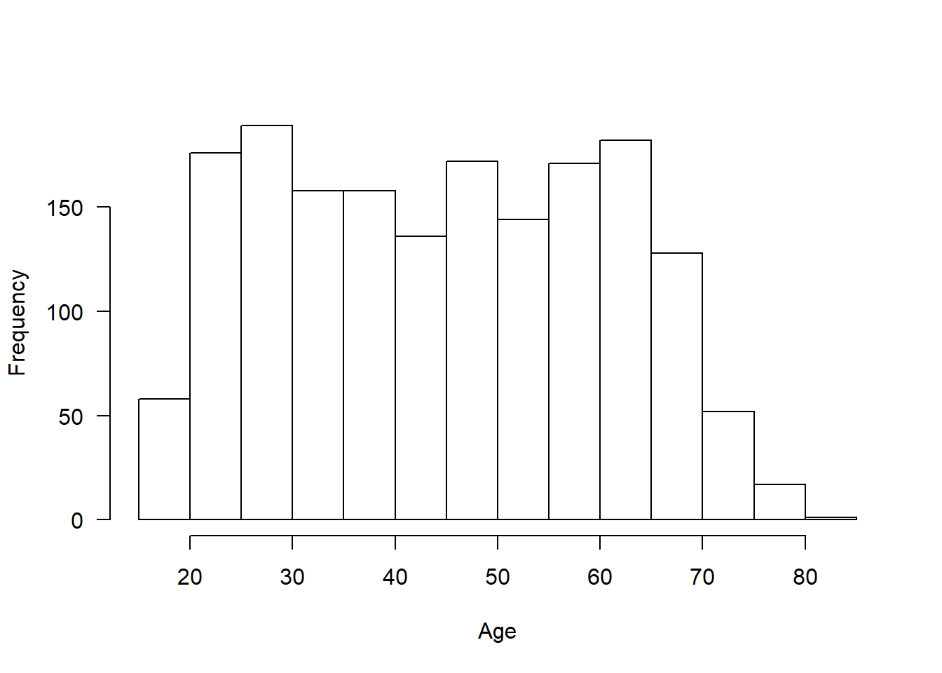
###############################################################################################################2.5 Summary of COVID related variables
How long have you been in “lockdown”?
hist(covfin$COVID_ndays_4, xlab="Days in `lockdown`",main="",las=1)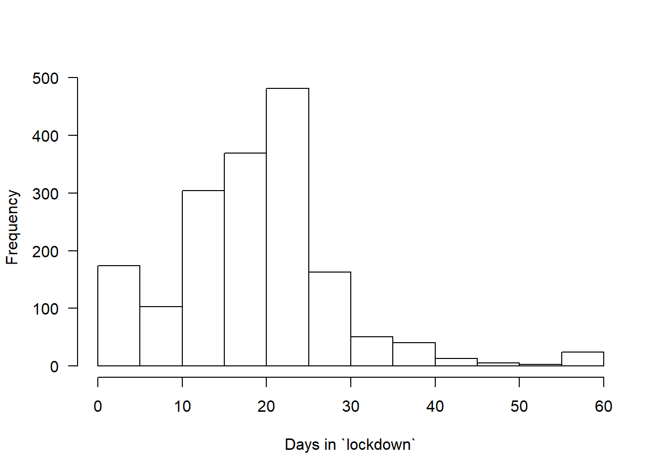
Have you, temporarily or permanently, lost your job as a consequence of the novel coronavirus (COVID-19) pandemic?
cro_tpct(covfin$COVID_lost_job) %>% set_caption("I have lost my job: Percentages")| I have lost my job: Percentages | |
| #Total | |
|---|---|
| I lost my job | |
| No | 79.7 |
| Yes | 20.3 |
| #Total cases | 1742 |
What is your main source of information about the novel coronavirus (COVID-19) pandemic?
cro_tpct(covfin$COVID_info_source) %>% set_caption("Information source: Percentages")| Information source: Percentages | |
| #Total | |
|---|---|
| Information source | |
| Newspaper (printed or online) | 32.4 |
| Social media | 21.2 |
| Friends/family | 2.2 |
| Radio | 2.6 |
| Television | 32.8 |
| Other | 8.8 |
| #Total cases | 1742 |
Have you tested positive for COVID?
cro_tpct(covfin$COVID_pos) %>% set_caption("I tested positive for COVID-19: Percentages") | I tested positive for COVID-19: Percentages | |
| #Total | |
|---|---|
| I tested positive to COVID | |
| No | 99.8 |
| Yes | 0.2 |
| #Total cases | 1740 |
Has someone you know tested positive for COVID?
cro_tpct(covfin$COVID_pos_others) %>% set_caption("Somebody I know tested positive for COVID-19: Percentages") | Somebody I know tested positive for COVID-19: Percentages | |
| #Total | |
|---|---|
| Tested pos someone I know | |
| Yes | 16.3 |
| No | 83.7 |
| #Total cases | 1741 |
There are 4 items probing people’s COVID risk perception:
- How severe do you think novel coronavirus (COVID-19) will be in the population as a whole?
- How harmful would it be for your health if you were to become infected with COVID-19?
- How concerned are you that you might become infected with COVID-19?
- How concerned are you that somebody you know might become infected with novel?
Provide snapshot of responses and correlations between items.
covvars<-gather(covfin %>% select(c(COVID_gen_harm,COVID_pers_harm,COVID_pers_concern,COVID_concern_oth)),factor_key = TRUE)
covvars$key <- factor(covvars$key,labels=c("General harm","Personal harm","Concern self","Concern others"))
covhisto <- ggplot(covvars, aes(value)) +
  theme_classic() +
  theme(panel.grid.minor.y = element_line(colour="lightgray", size=0.5),
        panel.grid.major.y = element_line(colour="darkgray", size=0.5),
        panel.grid.major.x = element_blank(),
        panel.border = element_rect(colour = "black", size=1, fill=NA)) +
  geom_histogram(bins = 5, color="darkblue", fill="lightblue") +
  xlab("Response") + ylab("Frequency") +
  facet_wrap(~key, scales = 'free_x',labeller=label_value)
ggsave("covhisto.pdf")
Saving 7 x 5 in imageprint(covhisto)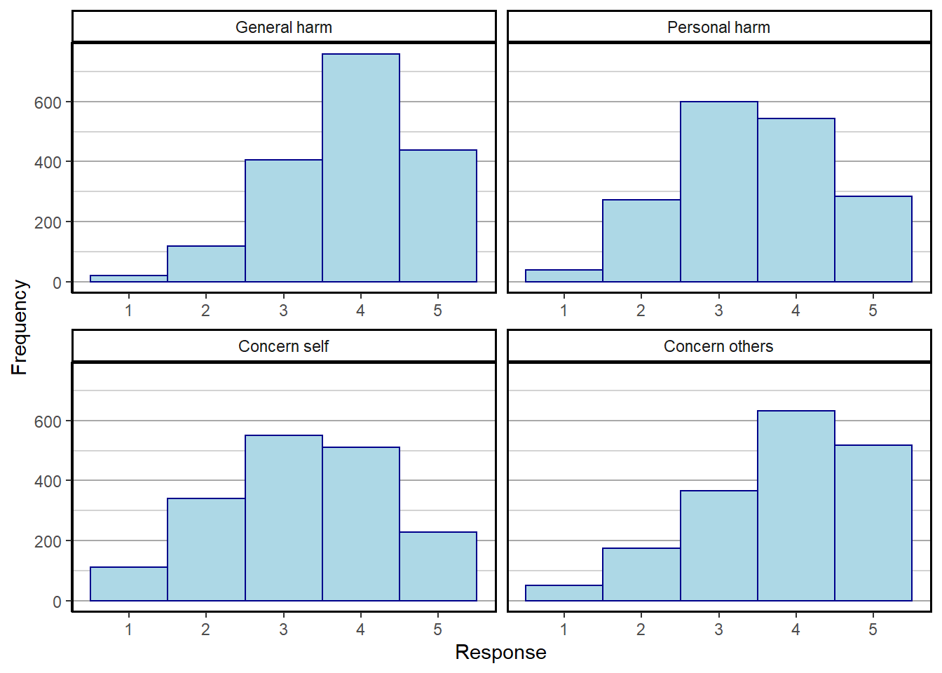
covfin %>% select(c(COVID_gen_harm,COVID_pers_harm,COVID_pers_concern,COVID_concern_oth)) %>% cor (.,use="pairwise.complete.obs") %>% round(.,3) COVID_gen_harm COVID_pers_harm COVID_pers_concern
COVID_gen_harm 1.000 0.473 0.493
COVID_pers_harm 0.473 1.000 0.578
COVID_pers_concern 0.493 0.578 1.000
COVID_concern_oth 0.520 0.421 0.695
COVID_concern_oth
COVID_gen_harm 0.520
COVID_pers_harm 0.421
COVID_pers_concern 0.695
COVID_concern_oth 1.000#compute composite score for COVID risk
covfin$COVIDrisk <- covfin %>% select(c(COVID_gen_harm,COVID_pers_harm,COVID_pers_concern,COVID_concern_oth)) %>% apply(.,1, mean, na.rm=TRUE)
#compute composite score for government trust
covfin$govtrust <- covfin %>% select(starts_with("trus")) %>% apply(.,1, mean, na.rm=TRUE)
###############################################################################################################3 Comparison between scenarios
3.1 Acceptability of policy
Not all items are entirely commensurate between scenarios. We begin with a graphical summary. The figure below shows people’s confidence that each of the scenarios would:
- reduce their likelihood of contracting COVID-19
- allow them to resume their normal lives more rapidly
- reduce spread of COVID-19 in the community.
#plot violins side by side
plotvn <- c("Reduce contracting","Resume normal","Reduce spread")
vioplot(select(covfin,c(reduce_lik_mild,return_activ_mild,reduce_spread_mild)), col = "yellow", plotCentre = "line", side = "left",
        las=1,names=plotvn,ylim=c(1,7.5))
vioplot(select(covfin,c(reduce_lik_sev,return_activ_sev,reduce_spread_severe)), col = "red", plotCentre = "line", side = "right", add = T )
title(xlab="Variable",ylab="Confidence")
legend(3,7.6, fill = c("yellow", "red"), legend = c("Mild", "Severe"), title = "Type of scenario")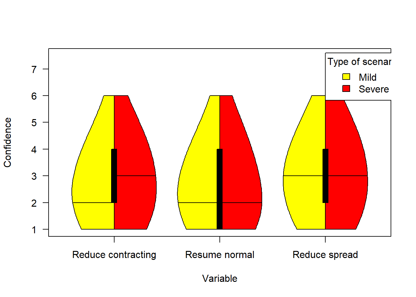
###############################################################################################################Basic acceptability of each scenario, probed by a single item immediately after reading the scenario. The table shows percentages. For the mild scenario, the question refers to whether participant would download the app. For the severe scenario, the question refers to acceptability of the tracking mandated by government.
covfin$accept1 <- apply(cbind(covfin$app_uptake1_mild,covfin$is_acceptable1_sev),1,sum,na.rm=TRUE)
covfin <- apply_labels(covfin,
                     accept1 = "Acceptability of policy",
                     accept1 = c("Yes" = 1, "No" = 0),
                     scenario_type = "Type of scenario")
cro_tpct(covfin$accept1,row_vars=covfin$scenario_type)| #Total | |||
|---|---|---|---|
| Type of scenario | |||
| mild | Acceptability of policy | No | 54.0 |
| Yes | 46.0 | ||
| #Total cases | 868 | ||
| severe | Acceptability of policy | No | 60.5 |
| Yes | 39.5 | ||
| #Total cases | 874 | ||
chisq.test(covfin$accept1,covfin$scenario_type,correct=TRUE)
    Pearson's Chi-squared test with Yates' continuity correction

data:  covfin$accept1 and covfin$scenario_type
X-squared = 7.2429, df = 1, p-value = 0.007118###############################################################################################################The difference between acceptability of scenarios is highly significant by a \(\chi^2\) test on the contingency table.
Repeated probing of basic acceptability of each scenario after multiple questions about the scenario have been answered. The table shows percentages. For the mild scenario, the question refers to whether participant would download the app. For the severe scenario, the question refers to acceptability of the tracking mandated by government.
covfin$accept2 <- apply(cbind(covfin$app_uptake2_mild,covfin$is_acceptable2_sev),1,sum,na.rm=TRUE)
covfin <- apply_labels(covfin,
                        accept2 = "Acceptability of policy",
                        accept2 = c("Yes" = 1, "No" = 0),
                        scenario_type = "Type of scenario")
cro_tpct(covfin$accept2,row_vars=covfin$scenario_type)| #Total | |||
|---|---|---|---|
| Type of scenario | |||
| mild | Acceptability of policy | No | 56.8 |
| Yes | 43.2 | ||
| #Total cases | 868 | ||
| severe | Acceptability of policy | No | 64.0 |
| Yes | 36.0 | ||
| #Total cases | 874 | ||
chisq.test(covfin$accept2,covfin$scenario_type,correct=TRUE)
    Pearson's Chi-squared test with Yates' continuity correction

data:  covfin$accept2 and covfin$scenario_type
X-squared = 9.0405, df = 1, p-value = 0.002641###############################################################################################################The difference between acceptability of scenarios is again significant by a \(\chi^2\) test, and overall acceptability of both scenarios has been reduced slightly compared to first set of questions.
Those people who found the scenario unacceptable at the second opportunity were asked two follow-up questions. Those questions were as follows:
First, for both scenarios, people were asked if their decision would change if the government was required to delete the data and cease tracking after 6 months. Responses to this sunset question (percentages) were as follows:
covfin$accept3 <- apply(cbind(covfin$accept2,covfin %>% select(contains("sunset"))),1,sum,na.rm=TRUE)
covfin <- apply_labels(covfin,
                       accept3 = "Acceptability of policy",
                       accept3 = c("Yes" = 1, "No" = 0),
                       scenario_type = "Type of scenario")
cro_tpct(covfin$accept3,row_vars=covfin$scenario_type)| #Total | |||
|---|---|---|---|
| Type of scenario | |||
| mild | Acceptability of policy | No | 44.8 |
| Yes | 55.2 | ||
| #Total cases | 868 | ||
| severe | Acceptability of policy | No | 50.0 |
| Yes | 50.0 | ||
| #Total cases | 874 | ||
chisq.test(covfin$accept3,covfin$scenario_type,correct=TRUE)
    Pearson's Chi-squared test with Yates' continuity correction

data:  covfin$accept3 and covfin$scenario_type
X-squared = 4.4889, df = 1, p-value = 0.03412###############################################################################################################The sunset clause increased acceptability of the scenario, although some opposition remained.
The second follow-up question differed between scenarios. People in the mild scenario were asked if they would change their decision if data was stored only on the user’s smartphone (not government servers), and people were given the option to provide the data if they tested positive. People in the severe scenario were asked if they would change their decision if there was an option to opt out of data collection.
covfin$accept5 <- apply(cbind(covfin$accept2,covfin %>% select(contains("sunset")),
                                      covfin$change_dlocal_mild,covfin$change_optout_sev),1,max,na.rm=TRUE)
covfin <- apply_labels(covfin,
                       accept5 = "Acceptability of policy",
                       accept5 = c("Yes" = 1, "No" = 0),
                       scenario_type = "Type of scenario")
cro_tpct(covfin$accept5,row_vars=covfin$scenario_type)| #Total | |||
|---|---|---|---|
| Type of scenario | |||
| mild | Acceptability of policy | No | 32.4 |
| Yes | 67.6 | ||
| #Total cases | 868 | ||
| severe | Acceptability of policy | No | 29.3 |
| Yes | 70.7 | ||
| #Total cases | 874 | ||
chisq.test(covfin$accept5,covfin$scenario_type,correct=TRUE)
    Pearson's Chi-squared test with Yates' continuity correction

data:  covfin$accept5 and covfin$scenario_type
X-squared = 1.7989, df = 1, p-value = 0.1798###############################################################################################################The opt-out/local storage options further enhanced acceptance.
3.2 Assessment of risk of scenarios, trust in government and data security
The next graph shows responses to the following items (abridged from survey):
- How difficult is it for people to decline participation in the proposed project? (1 = Extremely easy – 6 = Extremely difficult)
- To what extent is the Government only collecting the data necessary? (1 = Not at all – 6 = Completely)
- How sensitive is the data being collected in the proposed project? (1 = Not at all – 6 = Extremely)
- How serious is the risk of harm that could arise from the proposed project? (1 = Not at all – 6 = Extremely)
- How much do you trust the Government to use the tracking data only to deal with the COVID-19 pandemic? (1 = Not at all – 6 = Completely)
- How much do you trust the Government to be able to ensure the privacy of each individual? (1 = Not at all – 6 = Completely)
- How secure is the data that would be collected for the proposed project? (1 = Not at all – 6 = Completely)
- To what extent do people have ongoing control of their data? (1 = No control at all – 6 = Complete control)
#plot violins side by side
#x11(width=10,height=6)
plotvn <- c("Decline","Necessary","Sensitive","Risk","Trust use","Trust privacy","Secure", "Control")

vioplot(select(filter(covfin,scenario_type=="mild"),c(decline_participate:ongoing_control)), col = "yellow", plotCentre = "line", side = "left",
        las=1,names=plotvn,ylim=c(1,7.5))
vioplot(select(filter(covfin,scenario_type=="severe"),c(decline_participate:ongoing_control)), col = "red", plotCentre = "line", side = "right", add = T )
title(xlab="Variable",ylab="Response")
legend(3,7.6, fill = c("yellow", "red"), legend = c("Mild", "Severe"), title = "Type of scenario")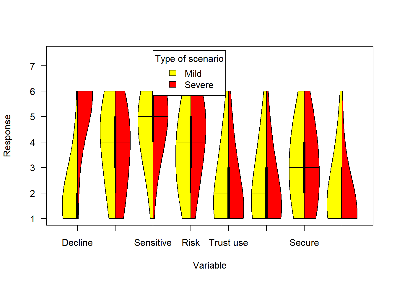
###############################################################################################################4 Role of worldviews
4.1 Worldview and risk perception
We relate a composite of the 3 worldview items to the composite of the 4 items probing perceived risk from COVID. Worldview is scored such that greater values reflect greater libertarianism.
p <- ggplot(covfin, aes(Worldview, COVIDrisk)) +
  geom_point(size=1.5,shape = 21,fill="red",
             position=position_jitter(width=0.15, height=0.15)) +
  geom_smooth() +
  theme(plot.title = element_text(size = 18),
        panel.background = element_rect(fill = "white", colour = "grey50"),
        text = element_text(size=14)) +
  xlim(0.8,7.2) + ylim(0.8,5.2) +
  labs(x="Worldview (libertarianism)", y="Perceived COVID risk")
print(p)
`geom_smooth()` using method = 'gam' and formula 'y ~ s(x, bs = "cs")'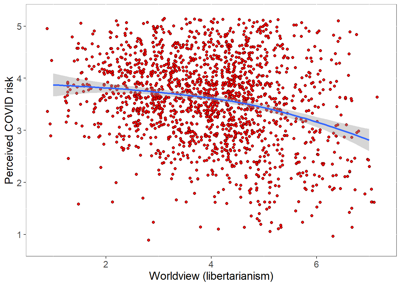
pcor <- cor.test (covfin$Worldview,covfin$COVIDrisk, use="pairwise.complete.obs") %>% print()
    Pearson's product-moment correlation

data:  covfin$Worldview and covfin$COVIDrisk
t = -9.9172, df = 1740, p-value < 2.2e-16
alternative hypothesis: true correlation is not equal to 0
95 percent confidence interval:
 -0.2752740 -0.1863578
sample estimates:
       cor
-0.2312988 ###############################################################################################################There is a moderately large and statistically highly significant correlation between worldviews and risk perception, such that greater libertarianism is associated with reduced risk perception. The variance accounted for (0.053) is small.
4.2 Worldviews and trust
We relate the composite of the 3 worldview items to the composite of the two trust-in-government items (which correlate 0.806).
p <- ggplot(covfin, aes(Worldview, govtrust)) +
  geom_point(size=1.5,shape = 21,fill="red",
             position=position_jitter(width=0.15, height=0.15)) +
  geom_smooth() +
  theme(plot.title = element_text(size = 18),
        panel.background = element_rect(fill = "white", colour = "grey50"),
        text = element_text(size=14)) +
  xlim(0.8,7.2) + ylim(0.8,5.2) +
  labs(x="Worldview (libertarianism)", y="Trust in government")
print(p)
`geom_smooth()` using method = 'gam' and formula 'y ~ s(x, bs = "cs")'Warning: Removed 29 rows containing non-finite values (stat_smooth).Warning: Removed 29 rows containing missing values (geom_point).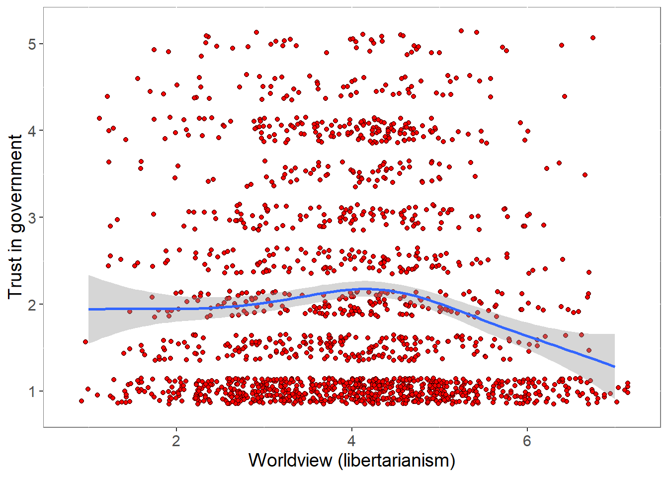
pcor <- cor.test (covfin$Worldview,covfin$govtrust, use="pairwise.complete.obs") %>% print()
    Pearson's product-moment correlation

data:  covfin$Worldview and covfin$govtrust
t = -2.124, df = 1740, p-value = 0.03381
alternative hypothesis: true correlation is not equal to 0
95 percent confidence interval:
 -0.097584777 -0.003896204
sample estimates:
        cor
-0.05085237 ###############################################################################################################The pattern is not straightforward and may not be linear, but there is some evidence that trust is reduced among extreme libertarians. The significant correlation must be interpreted with caution
5 Logistic modeling
We now try to model acceptability of the scenarios from some of the other variables using logistic regression. The models were initially developed by Dan Little, imported and extended by Stephan Lewandowsky on 7 April 2020.
5.1 Mixed-effects modeling
The first model is a mixed-effects model. This includes a random intercept (i.e., a different intercept for each participant). The model used the various trust variables and other questions about the policies being proposed.
lrmod1 <- glmer(accept1 ~ decline_participate + proportionality + sensitivity + risk_of_harm + trust_intentions + trust_respect_priv  + scenario_type + (1 | id),
                data = covfin %>% mutate(accept1=unlabel(accept1)) %>% mutate(scenario_type=unlabel(scenario_type)), family = binomial)
boundary (singular) fit: see ?isSingularsumm(lrmod1,digits=3)Warning in summ.merMod(lrmod1, digits = 3): Could not calculate r-squared. Try removing missing data
before fitting the model.| Observations | 1742 |
| Dependent variable | accept1 |
| Type | Mixed effects generalized linear model |
| Family | binomial |
| Link | logit |
| AIC | 1654.441 |
| BIC | 1703.606 |
| Est. | S.E. | z val. | p | |
|---|---|---|---|---|
| (Intercept) | -1.511 | 0.353 | -4.279 | 0.000 |
| decline_participate | -0.201 | 0.059 | -3.395 | 0.001 |
| proportionality | 0.181 | 0.044 | 4.120 | 0.000 |
| sensitivity | 0.009 | 0.059 | 0.148 | 0.883 |
| risk_of_harm | -0.330 | 0.050 | -6.546 | 0.000 |
| trust_intentions | 0.651 | 0.075 | 8.726 | 0.000 |
| trust_respect_priv | 0.314 | 0.073 | 4.277 | 0.000 |
| scenario_typesevere | 0.963 | 0.257 | 3.743 | 0.000 |
| Group | Parameter | Std. Dev. |
|---|---|---|
| id | (Intercept) | 0.000 |
| Group | # groups | ICC |
|---|---|---|
| id | 1742 | 0.000 |
#try a different optimizer to see if singularity persists
ss <- getME(lrmod1,c("theta","fixef"))
lrmod1a <- update(lrmod1,start=ss,control=glmerControl(optimizer="bobyqa",   optCtrl=list(maxfun=2e5)))
boundary (singular) fit: see ?isSingularsumm(lrmod1a,digits=3)Warning in summ.merMod(lrmod1a, digits = 3): Could not calculate r-squared. Try removing missing data
before fitting the model.| Observations | 1742 |
| Dependent variable | accept1 |
| Type | Mixed effects generalized linear model |
| Family | binomial |
| Link | logit |
| AIC | 1654.441 |
| BIC | 1703.606 |
| Est. | S.E. | z val. | p | |
|---|---|---|---|---|
| (Intercept) | -1.511 | 0.353 | -4.279 | 0.000 |
| decline_participate | -0.201 | 0.059 | -3.395 | 0.001 |
| proportionality | 0.181 | 0.044 | 4.120 | 0.000 |
| sensitivity | 0.009 | 0.059 | 0.148 | 0.883 |
| risk_of_harm | -0.330 | 0.050 | -6.546 | 0.000 |
| trust_intentions | 0.651 | 0.075 | 8.726 | 0.000 |
| trust_respect_priv | 0.314 | 0.073 | 4.277 | 0.000 |
| scenario_typesevere | 0.963 | 0.257 | 3.743 | 0.000 |
| Group | Parameter | Std. Dev. |
|---|---|---|
| id | (Intercept) | 0.000 |
| Group | # groups | ICC |
|---|---|---|
| id | 1742 | 0.000 |
#use composite score for trust
covfin$trust <- (covfin$proportionality + covfin$trust_intentions + covfin$trust_respect_priv)/3
lrmod1b <- glmer(accept1 ~ decline_participate +  sensitivity + risk_of_harm + trust  + scenario_type + (1 | id),
                 data = covfin %>% mutate(accept1=unlabel(accept1)) %>% mutate(scenario_type=unlabel(scenario_type)), family = binomial)
boundary (singular) fit: see ?isSingularsumm(lrmod1b,digits=3)Warning in summ.merMod(lrmod1b, digits = 3): Could not calculate r-squared. Try removing missing data
before fitting the model.| Observations | 1742 |
| Dependent variable | accept1 |
| Type | Mixed effects generalized linear model |
| Family | binomial |
| Link | logit |
| AIC | 1683.269 |
| BIC | 1721.509 |
| Est. | S.E. | z val. | p | |
|---|---|---|---|---|
| (Intercept) | -1.782 | 0.346 | -5.151 | 0.000 |
| decline_participate | -0.186 | 0.059 | -3.168 | 0.002 |
| sensitivity | -0.026 | 0.057 | -0.448 | 0.654 |
| risk_of_harm | -0.324 | 0.049 | -6.567 | 0.000 |
| trust | 1.134 | 0.068 | 16.718 | 0.000 |
| scenario_typesevere | 0.923 | 0.255 | 3.622 | 0.000 |
| Group | Parameter | Std. Dev. |
|---|---|---|
| id | (Intercept) | 0.000 |
| Group | # groups | ICC |
|---|---|---|
| id | 1742 | 0.000 |
###############################################################################################################It is clear that the singularity is caused by the near-zero random-effects variance and seems quite resistant to a few attempts to get around it. The remaining models therefore drop the random effect.
5.2 Ordinary logistic regression
5.2.1 Acceptance as a function of trust in government and perceived consequences of policies
The two models are for the two acceptance/uptake questions: The first model is for the first question early on in the study, and the second model is for the question provided later on, after all the various questions about trust and so on have been answered.
mod1 <- glm(accept1 ~ decline_participate + proportionality + sensitivity + risk_of_harm + trust_intentions + trust_respect_priv  + scenario_type,
            data = covfin %>% mutate(accept1=unlabel(accept1)) %>% mutate(scenario_type=unlabel(scenario_type)), family = binomial)
summ(mod1,digits=3)| Observations | 1742 |
| Dependent variable | accept1 |
| Type | Generalized linear model |
| Family | binomial |
| Link | logit |
| χ²(7) | 741.315 |
| Pseudo-R² (Cragg-Uhler) | 0.465 |
| Pseudo-R² (McFadden) | 0.312 |
| AIC | 1652.441 |
| BIC | 1696.144 |
| Est. | S.E. | z val. | p | |
|---|---|---|---|---|
| (Intercept) | -1.511 | 0.353 | -4.279 | 0.000 |
| decline_participate | -0.201 | 0.059 | -3.395 | 0.001 |
| proportionality | 0.181 | 0.044 | 4.120 | 0.000 |
| sensitivity | 0.009 | 0.059 | 0.148 | 0.883 |
| risk_of_harm | -0.330 | 0.050 | -6.546 | 0.000 |
| trust_intentions | 0.651 | 0.075 | 8.726 | 0.000 |
| trust_respect_priv | 0.314 | 0.073 | 4.277 | 0.000 |
| scenario_typesevere | 0.963 | 0.257 | 3.743 | 0.000 |
| Standard errors: MLE |
summ(mod1,digits=3,scale=TRUE)| Observations | 1742 |
| Dependent variable | accept1 |
| Type | Generalized linear model |
| Family | binomial |
| Link | logit |
| χ²(7) | 741.315 |
| Pseudo-R² (Cragg-Uhler) | 0.465 |
| Pseudo-R² (McFadden) | 0.312 |
| AIC | 1652.441 |
| BIC | 1696.144 |
| Est. | S.E. | z val. | p | |
|---|---|---|---|---|
| (Intercept) | -0.788 | 0.145 | -5.450 | 0.000 |
| decline_participate | -0.439 | 0.129 | -3.395 | 0.001 |
| proportionality | 0.291 | 0.071 | 4.120 | 0.000 |
| sensitivity | 0.010 | 0.071 | 0.148 | 0.883 |
| risk_of_harm | -0.506 | 0.077 | -6.546 | 0.000 |
| trust_intentions | 0.902 | 0.103 | 8.726 | 0.000 |
| trust_respect_priv | 0.422 | 0.099 | 4.277 | 0.000 |
| scenario_type | 0.963 | 0.257 | 3.743 | 0.000 |
| Standard errors: MLE; Continuous predictors are mean-centered and scaled by 1 s.d. |
plot_summs(mod1, scale = TRUE, plot.distributions = TRUE, inner_ci_level = .9)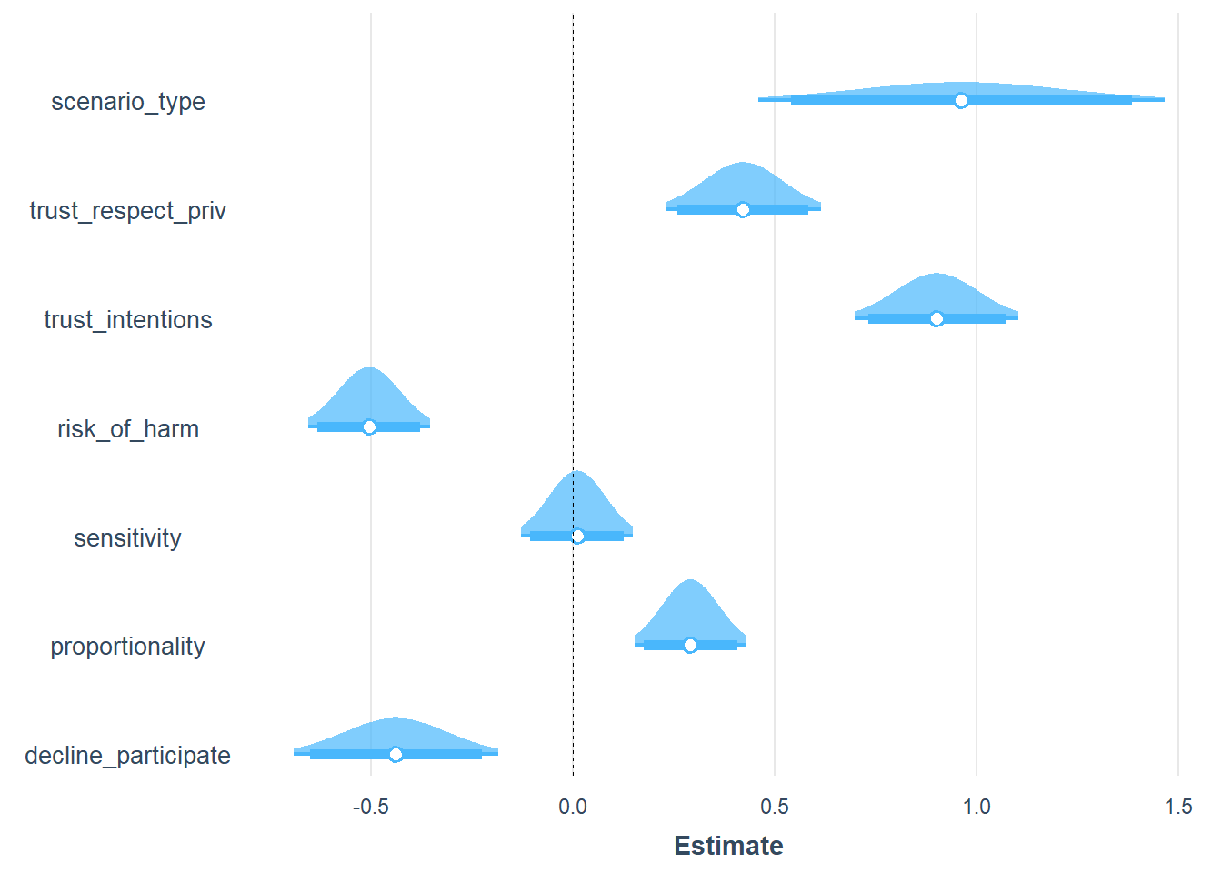
mod2 <- glm(accept2 ~ decline_participate + proportionality + sensitivity + risk_of_harm + trust_intentions + trust_respect_priv  +  scenario_type,
            data = covfin %>% mutate(accept2=unlabel(accept2)) %>% mutate(scenario_type=unlabel(scenario_type)), family = binomial)
summ(mod2,digits=3)| Observations | 1742 |
| Dependent variable | accept2 |
| Type | Generalized linear model |
| Family | binomial |
| Link | logit |
| χ²(7) | 794.654 |
| Pseudo-R² (Cragg-Uhler) | 0.496 |
| Pseudo-R² (McFadden) | 0.340 |
| AIC | 1560.494 |
| BIC | 1604.196 |
| Est. | S.E. | z val. | p | |
|---|---|---|---|---|
| (Intercept) | -1.790 | 0.362 | -4.939 | 0.000 |
| decline_participate | -0.115 | 0.061 | -1.893 | 0.058 |
| proportionality | 0.221 | 0.047 | 4.748 | 0.000 |
| sensitivity | -0.028 | 0.060 | -0.473 | 0.636 |
| risk_of_harm | -0.357 | 0.052 | -6.873 | 0.000 |
| trust_intentions | 0.665 | 0.074 | 8.939 | 0.000 |
| trust_respect_priv | 0.322 | 0.074 | 4.367 | 0.000 |
| scenario_typesevere | 0.631 | 0.263 | 2.396 | 0.017 |
| Standard errors: MLE |
summ(mod2,digits=3,scale=TRUE)| Observations | 1742 |
| Dependent variable | accept2 |
| Type | Generalized linear model |
| Family | binomial |
| Link | logit |
| χ²(7) | 794.654 |
| Pseudo-R² (Cragg-Uhler) | 0.496 |
| Pseudo-R² (McFadden) | 0.340 |
| AIC | 1560.494 |
| BIC | 1604.196 |
| Est. | S.E. | z val. | p | |
|---|---|---|---|---|
| (Intercept) | -0.843 | 0.149 | -5.648 | 0.000 |
| decline_participate | -0.252 | 0.133 | -1.893 | 0.058 |
| proportionality | 0.357 | 0.075 | 4.748 | 0.000 |
| sensitivity | -0.034 | 0.072 | -0.473 | 0.636 |
| risk_of_harm | -0.548 | 0.080 | -6.873 | 0.000 |
| trust_intentions | 0.921 | 0.103 | 8.939 | 0.000 |
| trust_respect_priv | 0.433 | 0.099 | 4.367 | 0.000 |
| scenario_type | 0.631 | 0.263 | 2.396 | 0.017 |
| Standard errors: MLE; Continuous predictors are mean-centered and scaled by 1 s.d. |
plot_summs(mod2, scale = TRUE, plot.distributions = TRUE, inner_ci_level = .9)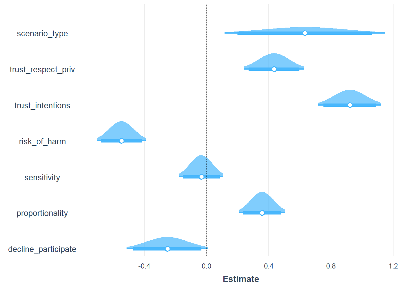
###############################################################################################################The type of scenario has a large effect. Acceptance increases with trust in government and declines with perceived risk of harm from the policy. The pattern is consistent across the two opportunities to express an opinion on acceptance.
5.2.2 Acceptance as a function of perceived severity of COVID
The models again target the two acceptance/uptake items in turn. The predictors are all the COVID-related items, including days in lockdown and job loss and so on.
mod3 <- glm(accept1 ~ COVID_gen_harm + COVID_pers_harm + COVID_pers_concern + COVID_concern_oth + COVID_pos + COVID_pos_others + COVID_ndays_4 + COVID_lost_job + scenario_type, data = covfin, family = binomial)
summ(mod3,digits=3)| Observations | 1728 (14 missing obs. deleted) |
| Dependent variable | accept1 |
| Type | Generalized linear model |
| Family | binomial |
| Link | logit |
| χ²(9) | 90.753 |
| Pseudo-R² (Cragg-Uhler) | 0.069 |
| Pseudo-R² (McFadden) | 0.038 |
| AIC | 2287.293 |
| BIC | 2341.840 |
| Est. | S.E. | z val. | p | |
|---|---|---|---|---|
| (Intercept) | -2.677 | 0.385 | -6.955 | 0.000 |
| COVID_gen_harm | 0.176 | 0.069 | 2.560 | 0.010 |
| COVID_pers_harm | 0.104 | 0.063 | 1.657 | 0.098 |
| COVID_pers_concern | 0.163 | 0.070 | 2.330 | 0.020 |
| COVID_concern_oth | 0.075 | 0.069 | 1.080 | 0.280 |
| COVID_pos | 0.302 | 1.020 | 0.297 | 0.767 |
| COVID_pos_others | 0.270 | 0.138 | 1.946 | 0.052 |
| COVID_ndays_4 | 0.010 | 0.005 | 1.993 | 0.046 |
| COVID_lost_job | -0.205 | 0.125 | -1.633 | 0.103 |
| scenario_typesevere | -0.260 | 0.100 | -2.602 | 0.009 |
| Standard errors: MLE |
summ(mod3,digits=3,scale=TRUE)| Observations | 1728 (14 missing obs. deleted) |
| Dependent variable | accept1 |
| Type | Generalized linear model |
| Family | binomial |
| Link | logit |
| χ²(9) | 90.753 |
| Pseudo-R² (Cragg-Uhler) | 0.069 |
| Pseudo-R² (McFadden) | 0.038 |
| AIC | 2287.293 |
| BIC | 2341.840 |
| Est. | S.E. | z val. | p | |
|---|---|---|---|---|
| (Intercept) | -0.370 | 0.139 | -2.658 | 0.008 |
| COVID_gen_harm | 0.161 | 0.063 | 2.560 | 0.010 |
| COVID_pers_harm | 0.106 | 0.064 | 1.657 | 0.098 |
| COVID_pers_concern | 0.180 | 0.077 | 2.330 | 0.020 |
| COVID_concern_oth | 0.079 | 0.074 | 1.080 | 0.280 |
| COVID_pos | 0.302 | 1.020 | 0.297 | 0.767 |
| COVID_pos_others | 0.270 | 0.138 | 1.946 | 0.052 |
| COVID_ndays_4 | 0.102 | 0.051 | 1.993 | 0.046 |
| COVID_lost_job | -0.205 | 0.125 | -1.633 | 0.103 |
| scenario_type | -0.260 | 0.100 | -2.602 | 0.009 |
| Standard errors: MLE; Continuous predictors are mean-centered and scaled by 1 s.d. |
###############################################################################################################People are more likely to accept policies if they perceive greater potential for societal harm and higher personal concern. Because there was a large effect of scenario type, we next explore interactions.
mod4 <- glm(accept1 ~ COVID_gen_harm + COVID_pers_harm + COVID_pers_concern + COVID_concern_oth + COVID_pos + COVID_pos_others +
              COVID_ndays_4 + COVID_lost_job + scenario_type + scenario_type:COVID_gen_harm + scenario_type:COVID_pers_concern,
            data = covfin, family = binomial)
summ(mod4,digits=3)| Observations | 1728 (14 missing obs. deleted) |
| Dependent variable | accept1 |
| Type | Generalized linear model |
| Family | binomial |
| Link | logit |
| χ²(11) | 96.933 |
| Pseudo-R² (Cragg-Uhler) | 0.073 |
| Pseudo-R² (McFadden) | 0.041 |
| AIC | 2285.113 |
| BIC | 2350.569 |
| Est. | S.E. | z val. | p | |
|---|---|---|---|---|
| (Intercept) | -3.109 | 0.453 | -6.862 | 0.000 |
| COVID_gen_harm | 0.194 | 0.092 | 2.105 | 0.035 |
| COVID_pers_harm | 0.104 | 0.063 | 1.642 | 0.100 |
| COVID_pers_concern | 0.272 | 0.090 | 3.024 | 0.002 |
| COVID_concern_oth | 0.076 | 0.069 | 1.090 | 0.276 |
| COVID_pos | 0.195 | 1.022 | 0.191 | 0.849 |
| COVID_pos_others | 0.270 | 0.139 | 1.941 | 0.052 |
| COVID_ndays_4 | 0.010 | 0.005 | 1.975 | 0.048 |
| COVID_lost_job | -0.211 | 0.126 | -1.675 | 0.094 |
| scenario_typesevere | 0.620 | 0.472 | 1.311 | 0.190 |
| COVID_gen_harm:scenario_typesevere | -0.044 | 0.128 | -0.344 | 0.731 |
| COVID_pers_concern:scenario_typesevere | -0.215 | 0.105 | -2.039 | 0.041 |
| Standard errors: MLE |
summ(mod4,digits=3,scale=TRUE)| Observations | 1728 (14 missing obs. deleted) |
| Dependent variable | accept1 |
| Type | Generalized linear model |
| Family | binomial |
| Link | logit |
| χ²(11) | 96.933 |
| Pseudo-R² (Cragg-Uhler) | 0.073 |
| Pseudo-R² (McFadden) | 0.041 |
| AIC | 2285.113 |
| BIC | 2350.569 |
| Est. | S.E. | z val. | p | |
|---|---|---|---|---|
| (Intercept) | -0.380 | 0.140 | -2.710 | 0.007 |
| COVID_gen_harm | 0.179 | 0.085 | 2.105 | 0.035 |
| COVID_pers_harm | 0.105 | 0.064 | 1.642 | 0.100 |
| COVID_pers_concern | 0.299 | 0.099 | 3.024 | 0.002 |
| COVID_concern_oth | 0.080 | 0.074 | 1.090 | 0.276 |
| COVID_pos | 0.195 | 1.022 | 0.191 | 0.849 |
| COVID_pos_others | 0.270 | 0.139 | 1.941 | 0.052 |
| COVID_ndays_4 | 0.101 | 0.051 | 1.975 | 0.048 |
| COVID_lost_job | -0.211 | 0.126 | -1.675 | 0.094 |
| scenario_type | -0.244 | 0.101 | -2.424 | 0.015 |
| COVID_gen_harm:scenario_type | -0.040 | 0.117 | -0.344 | 0.731 |
| COVID_pers_concern:scenario_type | -0.237 | 0.116 | -2.039 | 0.041 |
| Standard errors: MLE; Continuous predictors are mean-centered and scaled by 1 s.d. |
plot_summs(mod4, scale = TRUE, plot.distributions = TRUE, inner_ci_level = .9)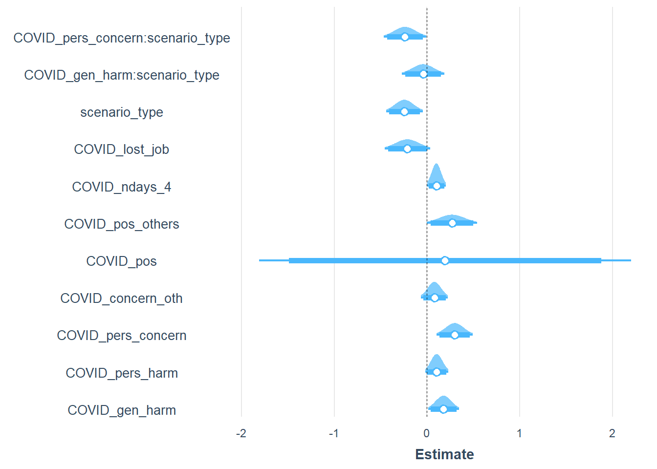
mod5 <- glm(accept2 ~ COVID_gen_harm + COVID_pers_harm + COVID_pers_concern + COVID_concern_oth + COVID_pos + COVID_pos_others + COVID_ndays_4 + COVID_lost_job + scenario_type + scenario_type:COVID_gen_harm + scenario_type:COVID_pers_concern, data = covfin, family = binomial)
summ(mod5,digits=3)| Observations | 1728 (14 missing obs. deleted) |
| Dependent variable | accept2 |
| Type | Generalized linear model |
| Family | binomial |
| Link | logit |
| χ²(11) | 76.835 |
| Pseudo-R² (Cragg-Uhler) | 0.059 |
| Pseudo-R² (McFadden) | 0.033 |
| AIC | 2266.281 |
| BIC | 2331.738 |
| Est. | S.E. | z val. | p | |
|---|---|---|---|---|
| (Intercept) | -2.605 | 0.448 | -5.815 | 0.000 |
| COVID_gen_harm | 0.112 | 0.092 | 1.218 | 0.223 |
| COVID_pers_harm | 0.077 | 0.064 | 1.213 | 0.225 |
| COVID_pers_concern | 0.273 | 0.090 | 3.037 | 0.002 |
| COVID_concern_oth | 0.064 | 0.070 | 0.920 | 0.358 |
| COVID_pos | 0.327 | 1.023 | 0.320 | 0.749 |
| COVID_pos_others | 0.181 | 0.139 | 1.297 | 0.195 |
| COVID_ndays_4 | 0.009 | 0.005 | 1.756 | 0.079 |
| COVID_lost_job | -0.148 | 0.126 | -1.173 | 0.241 |
| scenario_typesevere | 0.192 | 0.474 | 0.406 | 0.685 |
| COVID_gen_harm:scenario_typesevere | 0.057 | 0.129 | 0.443 | 0.657 |
| COVID_pers_concern:scenario_typesevere | -0.213 | 0.106 | -2.013 | 0.044 |
| Standard errors: MLE |
summ(mod5,digits=3,scale=TRUE)| Observations | 1728 (14 missing obs. deleted) |
| Dependent variable | accept2 |
| Type | Generalized linear model |
| Family | binomial |
| Link | logit |
| χ²(11) | 76.835 |
| Pseudo-R² (Cragg-Uhler) | 0.059 |
| Pseudo-R² (McFadden) | 0.033 |
| AIC | 2266.281 |
| BIC | 2331.738 |
| Est. | S.E. | z val. | p | |
|---|---|---|---|---|
| (Intercept) | -0.432 | 0.140 | -3.078 | 0.002 |
| COVID_gen_harm | 0.103 | 0.084 | 1.218 | 0.223 |
| COVID_pers_harm | 0.078 | 0.064 | 1.213 | 0.225 |
| COVID_pers_concern | 0.301 | 0.099 | 3.037 | 0.002 |
| COVID_concern_oth | 0.068 | 0.074 | 0.920 | 0.358 |
| COVID_pos | 0.327 | 1.023 | 0.320 | 0.749 |
| COVID_pos_others | 0.181 | 0.139 | 1.297 | 0.195 |
| COVID_ndays_4 | 0.090 | 0.052 | 1.756 | 0.079 |
| COVID_lost_job | -0.148 | 0.126 | -1.173 | 0.241 |
| scenario_type | -0.278 | 0.101 | -2.747 | 0.006 |
| COVID_gen_harm:scenario_type | 0.052 | 0.118 | 0.443 | 0.657 |
| COVID_pers_concern:scenario_type | -0.235 | 0.117 | -2.013 | 0.044 |
| Standard errors: MLE; Continuous predictors are mean-centered and scaled by 1 s.d. |
plot_summs(mod5, scale = TRUE, plot.distributions = TRUE, inner_ci_level = .9)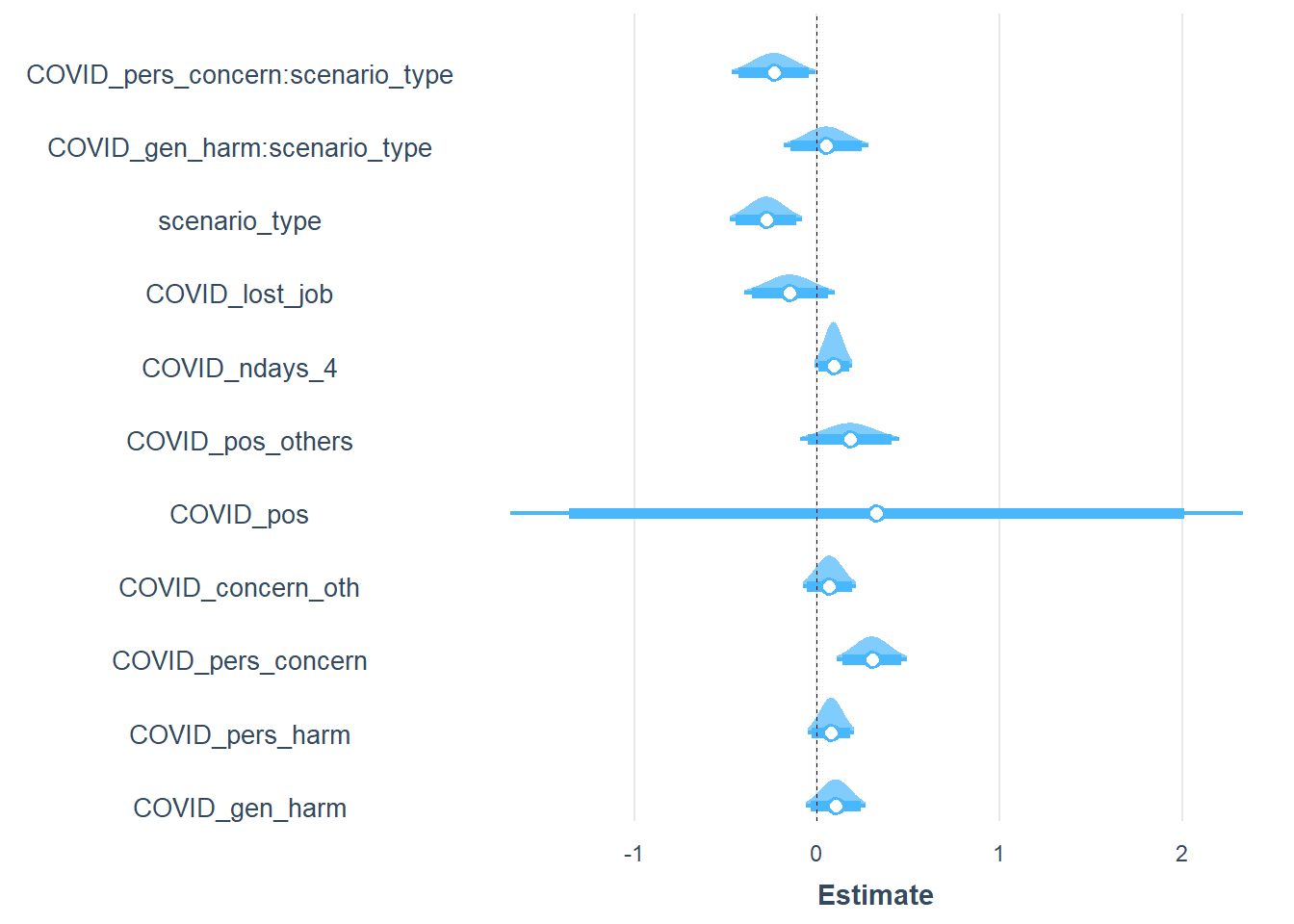
###############################################################################################################Perception of general severity marginally interacts with type of scenario. The borderline significance of the effect suggests it is not worth highlighting.
5.2.3 Full model for acceptance
The final model (for now) combines all predictors including Worldview composite.
mod6 <- glm(accept1 ~ COVID_gen_harm + COVID_pers_harm + COVID_pers_concern + COVID_concern_oth + COVID_pos + COVID_pos_others +
              COVID_ndays_4 + COVID_lost_job + scenario_type + scenario_type:COVID_gen_harm + scenario_type:COVID_pers_concern +
              decline_participate + proportionality + sensitivity + risk_of_harm + trust_intentions + trust_respect_priv +
              Worldview, data = covfin, family = binomial)
summ(mod6,digits=3)| Observations | 1728 (14 missing obs. deleted) |
| Dependent variable | accept1 |
| Type | Generalized linear model |
| Family | binomial |
| Link | logit |
| χ²(18) | 870.240 |
| Pseudo-R² (Cragg-Uhler) | 0.531 |
| Pseudo-R² (McFadden) | 0.369 |
| AIC | 1525.805 |
| BIC | 1629.445 |
| Est. | S.E. | z val. | p | |
|---|---|---|---|---|
| (Intercept) | -4.020 | 0.782 | -5.142 | 0.000 |
| COVID_gen_harm | 0.254 | 0.126 | 2.023 | 0.043 |
| COVID_pers_harm | 0.138 | 0.082 | 1.687 | 0.092 |
| COVID_pers_concern | 0.317 | 0.118 | 2.694 | 0.007 |
| COVID_concern_oth | 0.207 | 0.093 | 2.231 | 0.026 |
| COVID_pos | -1.446 | 1.352 | -1.070 | 0.285 |
| COVID_pos_others | 0.319 | 0.181 | 1.758 | 0.079 |
| COVID_ndays_4 | 0.016 | 0.007 | 2.419 | 0.016 |
| COVID_lost_job | -0.291 | 0.162 | -1.797 | 0.072 |
| scenario_typesevere | 3.544 | 0.704 | 5.036 | 0.000 |
| decline_participate | -0.203 | 0.062 | -3.268 | 0.001 |
| proportionality | 0.129 | 0.047 | 2.756 | 0.006 |
| sensitivity | -0.011 | 0.063 | -0.173 | 0.863 |
| risk_of_harm | -0.394 | 0.055 | -7.181 | 0.000 |
| trust_intentions | 0.693 | 0.079 | 8.731 | 0.000 |
| trust_respect_priv | 0.366 | 0.078 | 4.665 | 0.000 |
| Worldview | -0.357 | 0.060 | -5.978 | 0.000 |
| COVID_gen_harm:scenario_typesevere | -0.193 | 0.171 | -1.130 | 0.258 |
| COVID_pers_concern:scenario_typesevere | -0.508 | 0.138 | -3.677 | 0.000 |
| Standard errors: MLE |
summ(mod6,digits=3,scale=TRUE)| Observations | 1728 (14 missing obs. deleted) |
| Dependent variable | accept1 |
| Type | Generalized linear model |
| Family | binomial |
| Link | logit |
| χ²(18) | 870.240 |
| Pseudo-R² (Cragg-Uhler) | 0.531 |
| Pseudo-R² (McFadden) | 0.369 |
| AIC | 1525.805 |
| BIC | 1629.445 |
| Est. | S.E. | z val. | p | |
|---|---|---|---|---|
| (Intercept) | -1.176 | 0.219 | -5.367 | 0.000 |
| COVID_gen_harm | 0.233 | 0.115 | 2.023 | 0.043 |
| COVID_pers_harm | 0.140 | 0.083 | 1.687 | 0.092 |
| COVID_pers_concern | 0.350 | 0.130 | 2.694 | 0.007 |
| COVID_concern_oth | 0.220 | 0.099 | 2.231 | 0.026 |
| COVID_pos | -1.446 | 1.352 | -1.070 | 0.285 |
| COVID_pos_others | 0.319 | 0.181 | 1.758 | 0.079 |
| COVID_ndays_4 | 0.162 | 0.067 | 2.419 | 0.016 |
| COVID_lost_job | -0.291 | 0.162 | -1.797 | 0.072 |
| scenario_type | 1.158 | 0.272 | 4.258 | 0.000 |
| decline_participate | -0.444 | 0.136 | -3.268 | 0.001 |
| proportionality | 0.209 | 0.076 | 2.756 | 0.006 |
| sensitivity | -0.013 | 0.076 | -0.173 | 0.863 |
| risk_of_harm | -0.604 | 0.084 | -7.181 | 0.000 |
| trust_intentions | 0.957 | 0.110 | 8.731 | 0.000 |
| trust_respect_priv | 0.491 | 0.105 | 4.665 | 0.000 |
| Worldview | -0.427 | 0.071 | -5.978 | 0.000 |
| COVID_gen_harm:scenario_type | -0.178 | 0.157 | -1.130 | 0.258 |
| COVID_pers_concern:scenario_type | -0.560 | 0.152 | -3.677 | 0.000 |
| Standard errors: MLE; Continuous predictors are mean-centered and scaled by 1 s.d. |
plot_summs(mod6, scale = TRUE, plot.distributions = TRUE, inner_ci_level = .9)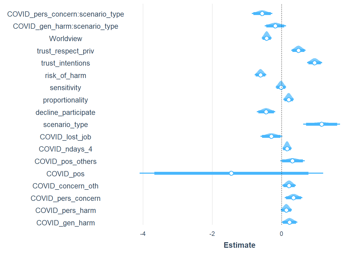
mod7 <- glm(accept2 ~ COVID_gen_harm + COVID_pers_harm + COVID_pers_concern + COVID_concern_oth + COVID_pos + COVID_pos_others +
              COVID_ndays_4 + COVID_lost_job + scenario_type + scenario_type:COVID_gen_harm + scenario_type:COVID_pers_concern +
              decline_participate + proportionality + sensitivity + risk_of_harm + trust_intentions + trust_respect_priv +
              Worldview, data = covfin, family = binomial)
summ(mod7,digits=3)| Observations | 1728 (14 missing obs. deleted) |
| Dependent variable | accept2 |
| Type | Generalized linear model |
| Family | binomial |
| Link | logit |
| χ²(18) | 888.253 |
| Pseudo-R² (Cragg-Uhler) | 0.544 |
| Pseudo-R² (McFadden) | 0.383 |
| AIC | 1468.864 |
| BIC | 1572.503 |
| Est. | S.E. | z val. | p | |
|---|---|---|---|---|
| (Intercept) | -3.548 | 0.785 | -4.518 | 0.000 |
| COVID_gen_harm | 0.106 | 0.128 | 0.832 | 0.405 |
| COVID_pers_harm | 0.091 | 0.084 | 1.088 | 0.277 |
| COVID_pers_concern | 0.339 | 0.121 | 2.800 | 0.005 |
| COVID_concern_oth | 0.202 | 0.095 | 2.113 | 0.035 |
| COVID_pos | -1.196 | 1.355 | -0.883 | 0.377 |
| COVID_pos_others | 0.179 | 0.185 | 0.967 | 0.334 |
| COVID_ndays_4 | 0.015 | 0.007 | 2.266 | 0.023 |
| COVID_lost_job | -0.171 | 0.165 | -1.036 | 0.300 |
| scenario_typesevere | 2.530 | 0.710 | 3.561 | 0.000 |
| decline_participate | -0.114 | 0.063 | -1.795 | 0.073 |
| proportionality | 0.177 | 0.049 | 3.601 | 0.000 |
| sensitivity | -0.051 | 0.064 | -0.805 | 0.421 |
| risk_of_harm | -0.410 | 0.056 | -7.339 | 0.000 |
| trust_intentions | 0.702 | 0.078 | 8.961 | 0.000 |
| trust_respect_priv | 0.360 | 0.078 | 4.635 | 0.000 |
| Worldview | -0.316 | 0.061 | -5.165 | 0.000 |
| COVID_gen_harm:scenario_typesevere | -0.013 | 0.176 | -0.074 | 0.941 |
| COVID_pers_concern:scenario_typesevere | -0.525 | 0.143 | -3.683 | 0.000 |
| Standard errors: MLE |
summ(mod7,digits=3,scale=TRUE)| Observations | 1728 (14 missing obs. deleted) |
| Dependent variable | accept2 |
| Type | Generalized linear model |
| Family | binomial |
| Link | logit |
| χ²(18) | 888.253 |
| Pseudo-R² (Cragg-Uhler) | 0.544 |
| Pseudo-R² (McFadden) | 0.383 |
| AIC | 1468.864 |
| BIC | 1572.503 |
| Est. | S.E. | z val. | p | |
|---|---|---|---|---|
| (Intercept) | -1.119 | 0.223 | -5.010 | 0.000 |
| COVID_gen_harm | 0.098 | 0.118 | 0.832 | 0.405 |
| COVID_pers_harm | 0.092 | 0.085 | 1.088 | 0.277 |
| COVID_pers_concern | 0.374 | 0.133 | 2.800 | 0.005 |
| COVID_concern_oth | 0.214 | 0.101 | 2.113 | 0.035 |
| COVID_pos | -1.196 | 1.355 | -0.883 | 0.377 |
| COVID_pos_others | 0.179 | 0.185 | 0.967 | 0.334 |
| COVID_ndays_4 | 0.155 | 0.069 | 2.266 | 0.023 |
| COVID_lost_job | -0.171 | 0.165 | -1.036 | 0.300 |
| scenario_type | 0.783 | 0.275 | 2.847 | 0.004 |
| decline_participate | -0.249 | 0.139 | -1.795 | 0.073 |
| proportionality | 0.286 | 0.079 | 3.601 | 0.000 |
| sensitivity | -0.062 | 0.077 | -0.805 | 0.421 |
| risk_of_harm | -0.628 | 0.086 | -7.339 | 0.000 |
| trust_intentions | 0.969 | 0.108 | 8.961 | 0.000 |
| trust_respect_priv | 0.484 | 0.104 | 4.635 | 0.000 |
| Worldview | -0.378 | 0.073 | -5.165 | 0.000 |
| COVID_gen_harm:scenario_type | -0.012 | 0.162 | -0.074 | 0.941 |
| COVID_pers_concern:scenario_type | -0.579 | 0.157 | -3.683 | 0.000 |
| Standard errors: MLE; Continuous predictors are mean-centered and scaled by 1 s.d. |
plot_summs(mod7, scale = TRUE, plot.distributions = TRUE, inner_ci_level = .9)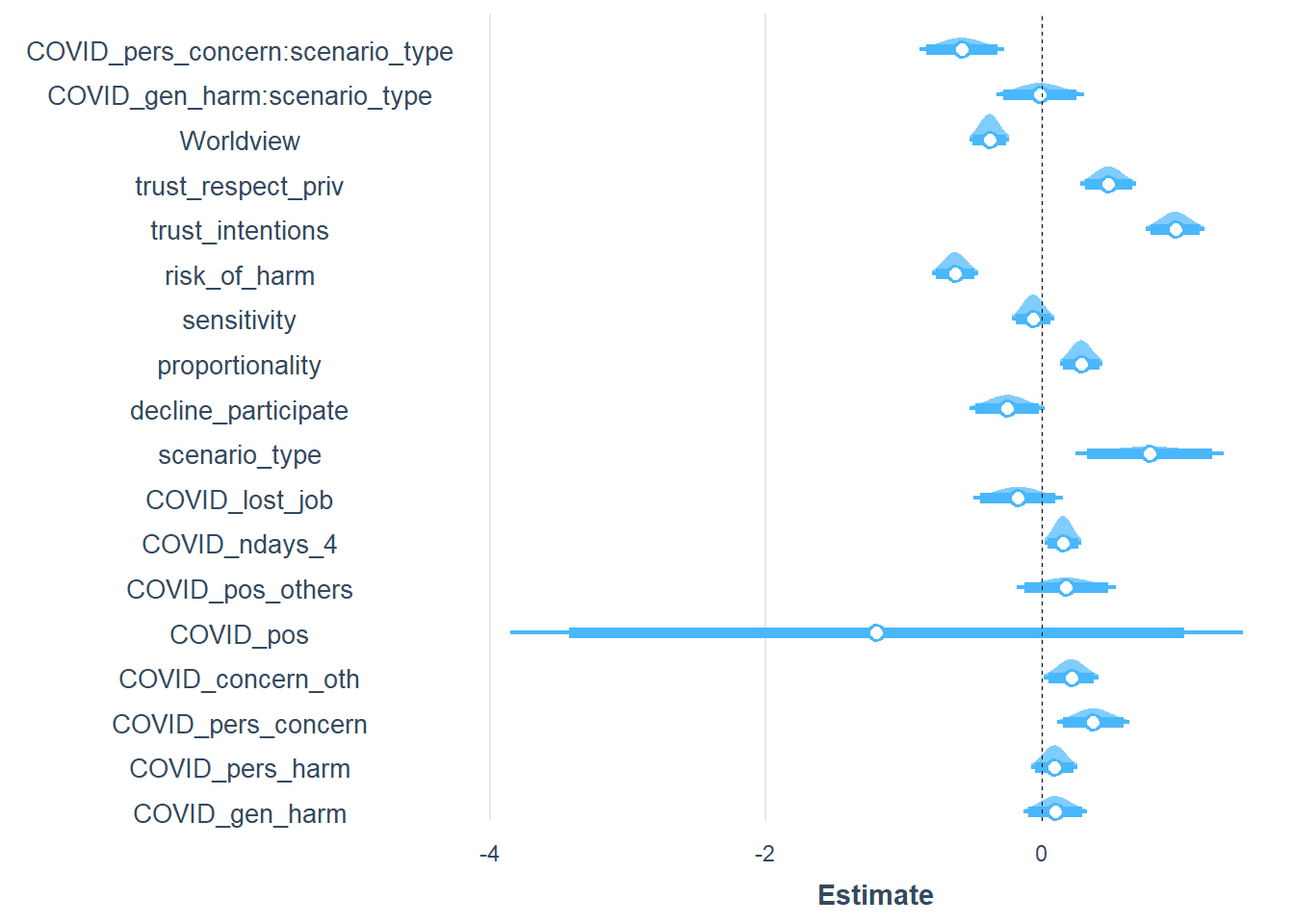
R version 3.6.3 (2020-02-29)
Platform: x86_64-w64-mingw32/x64 (64-bit)
Running under: Windows 10 x64 (build 19042)

Matrix products: default

locale:
[1] LC_COLLATE=English_United Kingdom.1252
[2] LC_CTYPE=English_United Kingdom.1252
[3] LC_MONETARY=English_United Kingdom.1252
[4] LC_NUMERIC=C
[5] LC_TIME=English_United Kingdom.1252

attached base packages:
[1] stats     graphics  grDevices utils     datasets  methods   base

other attached packages:
 [1] broom.mixed_0.2.4  kableExtra_1.2.1   jtools_2.0.3       expss_0.10.2
 [5] vioplot_0.3.4      zoo_1.8-7          sm_2.2-5.6         readxl_1.3.1
 [9] summarytools_0.9.6 scales_1.1.0       psych_1.9.12.31    reshape2_1.4.4
[13] Hmisc_4.4-0        Formula_1.2-3      survival_3.2-3     gridExtra_2.3
[17] lme4_1.1-21        Matrix_1.2-18      forcats_0.5.0      stringr_1.4.0
[21] dplyr_0.8.5        purrr_0.3.4        readr_1.3.1        tidyr_1.0.2
[25] tibble_3.0.1       ggplot2_3.3.0      tidyverse_1.3.0    stargazer_5.2.2
[29] hexbin_1.28.1      lattice_0.20-41    knitr_1.30         workflowr_1.6.1

loaded via a namespace (and not attached):
 [1] minqa_1.2.4         colorspace_1.4-1    pryr_0.1.4
 [4] ellipsis_0.3.0      rprojroot_1.3-2     ggstance_0.3.4
 [7] htmlTable_1.13.3    base64enc_0.1-3     fs_1.4.1
[10] rstudioapi_0.11     farver_2.0.3        fansi_0.4.1
[13] lubridate_1.7.8     xml2_1.3.2          codetools_0.2-16
[16] splines_3.6.3       mnormt_1.5-6        jsonlite_1.6.1
[19] nloptr_1.2.2.1      pbkrtest_0.4-8.6    broom_0.5.5
[22] cluster_2.1.0       dbplyr_1.4.2        png_0.1-7
[25] compiler_3.6.3      httr_1.4.1          backports_1.1.6
[28] assertthat_0.2.1    cli_2.0.2           later_1.0.0
[31] acepack_1.4.1       htmltools_0.4.0     tools_3.6.3
[34] lmerTest_3.1-2      coda_0.19-3         gtable_0.3.0
[37] glue_1.4.1          Rcpp_1.0.4.6        cellranger_1.1.0
[40] vctrs_0.2.4         nlme_3.1-145        xfun_0.20
[43] rvest_0.3.5         lifecycle_0.2.0     MASS_7.3-51.5
[46] hms_0.5.3           promises_1.1.0      parallel_3.6.3
[49] TMB_1.7.16          RColorBrewer_1.1-2  yaml_2.2.1
[52] pander_0.6.3        rpart_4.1-15        latticeExtra_0.6-29
[55] stringi_1.4.6       checkmate_2.0.0     boot_1.3-24
[58] rlang_0.4.6         pkgconfig_2.0.3     matrixStats_0.56.0
[61] evaluate_0.14       labeling_0.3        rapportools_1.0
[64] htmlwidgets_1.5.1   tidyselect_1.0.0    plyr_1.8.6
[67] magrittr_1.5        R6_2.4.1            magick_2.3
[70] generics_0.0.2      DBI_1.1.0           mgcv_1.8-31
[73] pillar_1.4.3        haven_2.2.0         whisker_0.4
[76] foreign_0.8-76      withr_2.2.0         nnet_7.3-13
[79] modelr_0.1.6        crayon_1.3.4        rmarkdown_2.6
[82] jpeg_0.1-8.1        grid_3.6.3          data.table_1.12.8
[85] git2r_0.26.1        webshot_0.5.2       reprex_0.3.0
[88] digest_0.6.25       numDeriv_2016.8-1.1 httpuv_1.5.2
[91] munsell_0.5.0       viridisLite_0.3.0   tcltk_3.6.3