United Kingdom Wave 2 on 16 April 2020
StephanLewandowsky
2020-04-17
Last updated: 2021-02-15
Checks: 7 0
Knit directory: UKsocialLicence/
This reproducible R Markdown analysis was created with workflowr (version 1.6.1). The Checks tab describes the reproducibility checks that were applied when the results were created. The Past versions tab lists the development history.
Great! Since the R Markdown file has been committed to the Git repository, you know the exact version of the code that produced these results.
Great job! The global environment was empty. Objects defined in the global environment can affect the analysis in your R Markdown file in unknown ways. For reproduciblity it’s best to always run the code in an empty environment.
The command set.seed(20200329) was run prior to running the code in the R Markdown file. Setting a seed ensures that any results that rely on randomness, e.g. subsampling or permutations, are reproducible.
Great job! Recording the operating system, R version, and package versions is critical for reproducibility.
Nice! There were no cached chunks for this analysis, so you can be confident that you successfully produced the results during this run.
Great job! Using relative paths to the files within your workflowr project makes it easier to run your code on other machines.
Great! You are using Git for version control. Tracking code development and connecting the code version to the results is critical for reproducibility.
The results in this page were generated with repository version 6da5a32. See the Past versions tab to see a history of the changes made to the R Markdown and HTML files.
Note that you need to be careful to ensure that all relevant files for the analysis have been committed to Git prior to generating the results (you can use wflow_publish or wflow_git_commit). workflowr only checks the R Markdown file, but you know if there are other scripts or data files that it depends on. Below is the status of the Git repository when the results were generated:
Ignored files:
    Ignored:    .Rhistory
    Ignored:    .Rproj.user/
    Ignored:    data/4 OSF Spain+social+licencing+COVID+Wave+1.csv
    Ignored:    data/4 OSF U.S.+social+licencing+COVID+Wave+1.csv
    Ignored:    data/4 OSF UK+social+licencing+Wave+2.csv
    Ignored:    data/4 OSF US varCovid.xlsx
    Ignored:    data/4 OSF varSpainCovid.xlsx
    Ignored:    data/4 OSF varUKCovidW2.xlsx
    Ignored:    data/Lucid SES info Spain 1.xlsx
    Ignored:    data/Spain+social+licencing+COVID+Wave+1.csv
    Ignored:    data/U.S.+social+licencing+COVID+Wave+1.csv
    Ignored:    data/UK early data covid 1st 500/
    Ignored:    data/UK+social+licencing+COVID+Wave+2.csv
    Ignored:    data/dupsUK.dat
    Ignored:    data/dupsUK2.dat
    Ignored:    data/dupsUS.dat
    Ignored:    data/varSpainCovid.xlsx
    Ignored:    data/varUKCovid.xlsx
    Ignored:    data/varUKCovidW2.xlsx
    Ignored:    data/varUSCovid.xlsx
    Ignored:    data/varnamediffs.csv

Untracked files:
    Untracked:  analysis/Paul's code/
    Untracked:  covhisto.pdf
Note that any generated files, e.g. HTML, png, CSS, etc., are not included in this status report because it is ok for generated content to have uncommitted changes.
These are the previous versions of the repository in which changes were made to the R Markdown (analysis/UKCovWave2.Rmd) and HTML (docs/UKCovWave2.html) files. If you’ve configured a remote Git repository (see ?wflow_git_remote), click on the hyperlinks in the table below to view the files as they were in that past version.
| File | Version | Author | Date | Message |
|---|---|---|---|---|
| html | 5bd9045 | StephanLewandowsky | 2021-02-05 | Build site. |
| html | bb03a95 | StephanLewandowsky | 2020-11-16 | Build site. |
| html | 7a92223 | StephanLewandowsky | 2020-11-15 | Build site. |
| html | fd1e250 | StephanLewandowsky | 2020-09-30 | Build site. |
| html | d6c4ad2 | StephanLewandowsky | 2020-07-28 | Build site. |
| html | 680986f | StephanLewandowsky | 2020-07-06 | Build site. |
| Rmd | 4f64552 | StephanLewandowsky | 2020-07-06 | wflow_publish(c(“analysis/index.Rmd”, “analysis/UKcov1.Rmd”, |
| html | 4f64552 | StephanLewandowsky | 2020-07-06 | wflow_publish(c(“analysis/index.Rmd”, “analysis/UKcov1.Rmd”, |
| html | 75ee0b1 | StephanLewandowsky | 2020-06-12 | Build site. |
| Rmd | ec9704c | StephanLewandowsky | 2020-06-12 | wflow_publish(c(“analysis/index.Rmd”, “analysis/UKcov1.Rmd”, |
| html | ec9704c | StephanLewandowsky | 2020-06-12 | wflow_publish(c(“analysis/index.Rmd”, “analysis/UKcov1.Rmd”, |
| html | 4841846 | StephanLewandowsky | 2020-05-20 | Build site. |
| html | 0937f8f | StephanLewandowsky | 2020-05-11 | Build site. |
| html | 2994975 | StephanLewandowsky | 2020-05-09 | Build site. |
| html | 7b7609a | StephanLewandowsky | 2020-05-07 | Build site. |
| html | a6c93f1 | StephanLewandowsky | 2020-05-06 | Build site. |
| Rmd | da4f46b | StephanLewandowsky | 2020-05-06 | wflow_publish(c(“analysis/index.Rmd”, “analysis/UKcov1.Rmd”, |
| html | da4f46b | StephanLewandowsky | 2020-05-06 | wflow_publish(c(“analysis/index.Rmd”, “analysis/UKcov1.Rmd”, |
| html | 7b6f263 | StephanLewandowsky | 2020-05-05 | Build site. |
| Rmd | bce7b96 | StephanLewandowsky | 2020-05-05 | wflow_publish(c(“analysis/index.Rmd”, “analysis/UKcov1.Rmd”, |
| html | bce7b96 | StephanLewandowsky | 2020-05-05 | wflow_publish(c(“analysis/index.Rmd”, “analysis/UKcov1.Rmd”, |
| html | bfd84e0 | StephanLewandowsky | 2020-05-05 | Build site. |
| Rmd | 3504379 | StephanLewandowsky | 2020-05-05 | wflow_publish(c(“analysis/index.Rmd”, “analysis/UKcov1.Rmd”, |
| html | 3504379 | StephanLewandowsky | 2020-05-05 | wflow_publish(c(“analysis/index.Rmd”, “analysis/UKcov1.Rmd”, |
| html | c656f8d | StephanLewandowsky | 2020-05-05 | Build site. |
| html | 641e4c5 | StephanLewandowsky | 2020-05-05 | Build site. |
| Rmd | e7cfb3d | StephanLewandowsky | 2020-05-05 | wflow_publish(c(“analysis/index.Rmd”, “analysis/UKcov1.Rmd”, |
| html | e7cfb3d | StephanLewandowsky | 2020-05-05 | wflow_publish(c(“analysis/index.Rmd”, “analysis/UKcov1.Rmd”, |
| html | 8061134 | StephanLewandowsky | 2020-04-27 | Build site. |
| html | 8370270 | StephanLewandowsky | 2020-04-26 | Build site. |
| Rmd | 0f0cdf3 | StephanLewandowsky | 2020-04-26 | wflow_publish(c(“analysis/index.Rmd”, “analysis/UKcov1.Rmd”, |
| html | 0f0cdf3 | StephanLewandowsky | 2020-04-26 | wflow_publish(c(“analysis/index.Rmd”, “analysis/UKcov1.Rmd”, |
| html | 33b991d | StephanLewandowsky | 2020-04-19 | Build site. |
| html | fdb4ddc | StephanLewandowsky | 2020-04-17 | Build site. |
| Rmd | 00910c1 | StephanLewandowsky | 2020-04-17 | wflow_publish(c(“analysis/index.Rmd”, “analysis/UKcov1.Rmd”, |
| html | 00910c1 | StephanLewandowsky | 2020-04-17 | wflow_publish(c(“analysis/index.Rmd”, “analysis/UKcov1.Rmd”, |
| html | e4874ce | StephanLewandowsky | 2020-04-17 | Build site. |
| Rmd | 0a8a791 | StephanLewandowsky | 2020-04-17 | wflow_publish(c(“analysis/index.Rmd”, “analysis/UKcov1.Rmd”, |
| html | 0a8a791 | StephanLewandowsky | 2020-04-17 | wflow_publish(c(“analysis/index.Rmd”, “analysis/UKcov1.Rmd”, |
| html | a1a91ec | StephanLewandowsky | 2020-04-17 | Build site. |
| Rmd | 41469ac | StephanLewandowsky | 2020-04-17 | wflow_publish(c(“analysis/index.Rmd”, “analysis/UKcov1.Rmd”, |
| html | 41469ac | StephanLewandowsky | 2020-04-17 | wflow_publish(c(“analysis/index.Rmd”, “analysis/UKcov1.Rmd”, |
| html | 3149892 | StephanLewandowsky | 2020-04-17 | Build site. |
| Rmd | bf52830 | StephanLewandowsky | 2020-04-17 | wflow_publish(c(“analysis/index.Rmd”, “analysis/UKcov1.Rmd”, |
| Rmd | 5e04926 | StephanLewandowsky | 2020-04-17 | intermittent update of code before knitting. |
1 Status of this report
These results represent a snapshot of an ongoing analysis and have not been peer-reviewed. They are for information but not for citation or to inform policy (as yet). Please report comments or bugs to stephan.lewandowsky@bristol.ac.uk or leave a comment on the relevant post on our subreddit.
Last update: Mon Feb 15 13:48:37 2021
These results are for the United Kingdom only, and are from a second wave of the stury. For other countries, return Home (click menu option on top) and choose another country. This work was supported by the Elizabeth Blackwell Institute, University of Bristol, with funding from the University’s alumni and friends.
In addition to the two scenarios (mild and severe) included in the first wave, this wave also included a Bluetooth scenario. The Bluetooth scenario was as follows:
Tracking COVID-19 Transmission
The COVID-19 pandemic has rapidly become a worldwide threat. Containing the virus’ spread is essential to minimise the impact on the healthcare system, the economy, and save many lives. Apple and Google have proposed adding a contact tracing capability to existing smartphones to help inform people if they have been exposed to others with COVID-19. This would help reduce community spread of COVID-19 by allowing people to voluntarily self-isolate. When two people are near each other, their phones would connect via bluetooth. If a person is later identified as being infected, the people they have been in close proximity to are then notified without the government knowing who they are. The use of this contact tracing capability would be completely voluntary. People who are notified would not be informed who had tested positive.
Participants: A representative samples of 1,500 U.K. participants were recruited on 16 April 2020. through the online platform Prolific. Participants were at least 18 years old. Participants were paid GBP 1.34 for their participation in the (approximately) 15-minute study. This worked out to be equivalent to GBP 5.98 per hour based on the average completion time.
Preregistration: The preregistration for the first wave of this study is here. It contains multiple files (under the Files menu), including the text of the preregistration and a copy of the Qualtrics source code for the first wave in the U.K. The survey used for this second wave is different and is available here (not preregistered).
Data: The data are available here. Note that demographics and other variables (such as location information and Prolific ID) that could lead to deanonymization have been omitted from the published data set. The results reported here include summaries of some of those variables.
2 Basic exploration
Note that the R code for this analysis can be hidden or made visible by clicking the black toggles next to each segment.
2.1 Setup and read data
Records 1 and 2 of the original file were transposed into columns in a new Excel file, called varUKCovidW2.xlsx, which therefore summarizes the short variable names (column 1, manually labelled varname) and the accompanying full text of the item (column 2, labelled fullname). Lines 2 and 3, which contain extended variable information, were then manually deleted from the .csv file provided by Qualtrics to facilitate reading of the file. The first two data records were also manually removed as they represented previews and tests from the preceding day.
In a non-public analysis of the raw data file, duplicate Prolific ID numbers (N=1) were identified and written to a text file for removal.
# Reading data and variable names
covfn        <- paste(inputdir,"UK+social+licencing+COVID+Wave+2.csv",sep="/") #this is the complete data file with demographics (but no location and IP). Version on OSF does not have demographics to reduce likelihood of reidentification of respondents.
covdata      <- read.csv(covfn)
#fix annoying misspelling of variables
covdata %<>% rename(wv_freemarket_lim = wv_.freemarket_lim, age_1 = age_4)
#read the duplicate records previously computed from the raw data set
duplicaterecs <- read.table(paste(inputdir,"dupsUK2.dat",sep="/"))
#which attention check options are correct
corattcheck<-c(1,1)
2.2 Clean up data
- Remove duplicate observations identified in a prior, private analysis.
- Remove observations that are returned as not having finished.
- Remove observations with a Status other than 0 (e.g., previews or suspected spam responses).
- Remove observations from participants who answered the fact check about the scenario incorrectly.
- Remove lots of unnecessary variables to create a lean dataset.
- Reverse score item wv_freemarket_lim so it points towards increasing libertarianism, just like the other two worldview items.
# from here on the code is identical between waves and countries, and hence there is not much in the .Rmd files.
# all the action takes place here

# remove duplicates first because the data set has not been touched yet, so the row pointers are correct
if (!is.null(duplicaterecs)) {
  covdata <- covdata [-unlist(duplicaterecs),]
}
covdata$attok <- covdata %>% select(starts_with("att_check")) %>% apply(.,1,FUN=function(x) sum(x==corattcheck,na.rm=TRUE)) #works for 1 or more attention checks
covfin  <- covdata %>% filter(Finished>0) %>% filter(attok == 1) %>%
                                              select(-c(starts_with("Recipient"),starts_with("Q_"),
                                                        Status,Finished,Progress,DistributionChannel,UserLanguage,
                                                        ResponseId,ExternalReference))
covfin$id <- 1:nrow(covfin)
covfin$scenario_type <- factor(covfin$scenario_type)  #get rid of empty levels (in case of Spain, those may have arisen through merge)


#create good labels for variables (from expss package)
#some of these are moved to each .Rmd file because different countries/waves have different labels for some items
covfin <- apply_labels(covfin,
                       gender = "Gender",
                       gender = c("Male" = 1, "Female" = 2, "Other" = 3, "Prefer not to say" =4),
                       COVID_pos = "I tested positive to COVID",
                       COVID_pos = c("Yes" = 1, "No" = 0),
                       scenario_type = "Type of policy scenario",
                       COVID_lost_job = "I lost my job",
                       COVID_lost_job = c("Yes" = 1, "No" = 0))


###############################################################################################################
#labels for country-specific variables
covfin <- apply_labels(covfin,
education = "Education",
education = c("GCSE" = 1, "A levels/VCE" = 2, "Apprent/Vocatnl" = 3, "University" = 4),
COVID_pos_others = "Tested pos someone I know",
COVID_pos_others = c("Yes" = 1, "No" = 0),
COVID_info_source= "Information source",
COVID_info_source = c("Newspaper (printed or online)" = 1, "Social media" = 2, "Friends/family" = 3, "Radio" = 4,
"Television" = 5, "Other" = 6, "Do not follow" = 7),
COVID_comply_pers = "Personal compliance",
COVID_comply_pers = c("I don't follow these policies at all" = 1,
"I mostly don't follow these policies"= 2,
"I follow these policies somewhat" = 3,
"I mostly follow these policies, but not all the way" = 4,
"I completely follow these policies" = 5,
"I go slightly beyond what the government policy mandates" = 6,
"I go somewhat beyond what the government policy mandates" = 7,
"I go significantly beyond what the government policy mandates" = 8,
"I am in complete quarantine and never leave my home" = 9),
mobileuse_sev = "Use mobile",
mobileuse_sev = c("Yes" = 1, "No" = 0),
smartphoneuse_mildbt = "Use smartphone",
smartphoneuse_mildbt = c("Yes" = 1, "No" = 0))
#reverse score
covfin <- covfin %>% mutate(wv_freemarket_lim=revscore(wv_freemarket_lim,7))
#compute composite score for worldview
covfin$Worldview <- covfin %>% select(starts_with("wv_")) %>% apply(.,1, mean, na.rm=TRUE)2.3 Demographics
Number of retained participants: 1446.
Gender, education, and age:
cro_tpct(covfin$gender) %>% set_caption("Gender identification: Percentages")| Gender identification: Percentages | |
| #Total | |
|---|---|
| Gender | |
| Male | 48.2 |
| Female | 51.7 |
| Other | 0.1 |
| Prefer not to say | 0.1 |
| #Total cases | 1446 |
cro_tpct(covfin$education) %>% set_caption("Level of education: Percentages")| Level of education: Percentages | |
| #Total | |
|---|---|
| Education | |
| GCSE | 14.6 |
| A levels/VCE | 17.2 |
| Apprent/Vocatnl | 11.8 |
| University | 56.4 |
| #Total cases | 1446 |
descr(covfin$age_1)Descriptive Statistics
covfin$age_1
N: 1446
age_1
----------------- ---------
Mean 46.15
Std.Dev 15.32
Min 18.00
Q1 32.00
Median 46.50
Q3 60.00
Max 87.00
MAD 20.02
IQR 28.00
CV 0.33
Skewness -0.05
SE.Skewness 0.06
Kurtosis -1.17
N.Valid 1446.00
Pct.Valid 100.00hist(covfin$age_1, xlab="Age",main="",las=1)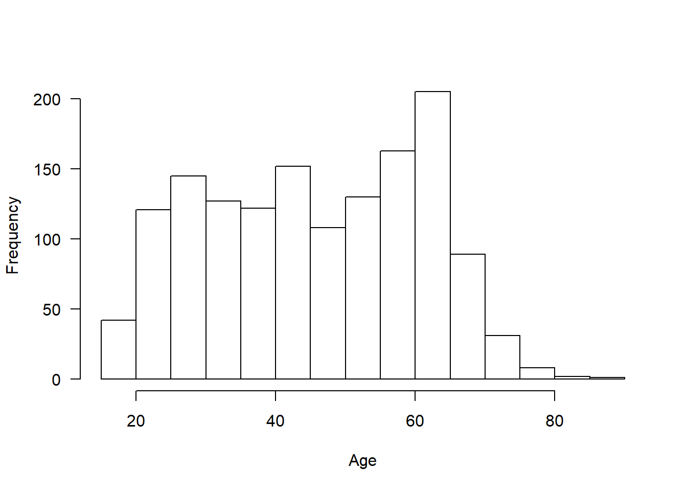
###############################################################################################################Phone ownership:
cro_tpct(covfin$smartphoneuse_mildbt) %>% set_caption("I use a smartphone: Percentages")| I use a smartphone: Percentages | |
| #Total | |
|---|---|
| Use smartphone | |
| No | 4.3 |
| Yes | 95.7 |
| #Total cases | 960 |
cro_tpct(covfin$mobileuse_sev) %>% set_caption("I use a mobile phone: Percentages")| I use a mobile phone: Percentages | |
| #Total | |
|---|---|
| Use mobile | |
| No | 1.4 |
| Yes | 98.6 |
| #Total cases | 486 |
2.4 COVID impact on participant
How long have you been in “lockdown”?
hist(covfin$COVID_ndays_4, xlab="Days in `lockdown`",main="",las=1)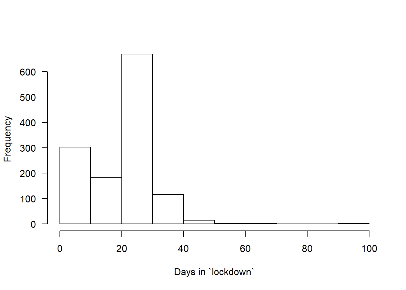
Have you, temporarily or permanently, lost your job as a consequence of the novel coronavirus (COVID-19) pandemic?
cro_tpct(covfin$COVID_lost_job) %>% set_caption("I have lost my job: Percentages")| I have lost my job: Percentages | |
| #Total | |
|---|---|
| I lost my job | |
| No | 83.5 |
| Yes | 16.5 |
| #Total cases | 1446 |
What is your main source of information about the novel coronavirus (COVID-19) pandemic?
cro_tpct(covfin$COVID_info_source) %>% set_caption("Information source: Percentages")| Information source: Percentages | |
| #Total | |
|---|---|
| Information source | |
| Newspaper (printed or online) | 29.3 |
| Social media | 10.0 |
| Friends/family | 1.2 |
| Radio | 5.5 |
| Television | 47.6 |
| Other | 5.4 |
| Do not follow | 1.1 |
| #Total cases | 1446 |
Have you tested positive for COVID?
cro_tpct(covfin$COVID_pos) %>% set_caption("I tested positive for COVID-19: Percentages") | I tested positive for COVID-19: Percentages | |
| #Total | |
|---|---|
| I tested positive to COVID | |
| No | 99.9 |
| Yes | 0.1 |
| #Total cases | 1446 |
Has someone you know tested positive for COVID?
cro_tpct(covfin$COVID_pos_others) %>% set_caption("Somebody I know tested positive for COVID-19: Percentages") | Somebody I know tested positive for COVID-19: Percentages | |
| #Total | |
|---|---|
| Tested pos someone I know | |
| No | 78.8 |
| Yes | 21.2 |
| #Total cases | 1446 |
What percentage of the population do you think is complying with government policies regarding social distancing?
hist(covfin$COVID_comply_percent,las=1,xlab="Estimated compliance of population (%)",main="")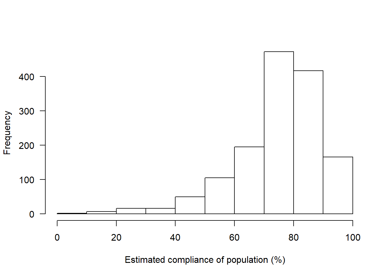
How much are you following government policies regarding social distancing?
cro_tpct(covfin$COVID_comply_pers) %>% set_caption("Compliance with policy: Percentages") | Compliance with policy: Percentages | |
| #Total | |
|---|---|
| Personal compliance | |
| I don’t follow these policies at all | 0.1 |
| I mostly don’t follow these policies | 0.6 |
| I follow these policies somewhat | 1.2 |
| I mostly follow these policies, but not all the way | 11.5 |
| I completely follow these policies | 58.0 |
| I go slightly beyond what the government policy mandates | 8.4 |
| I go somewhat beyond what the government policy mandates | 7.5 |
| I go significantly beyond what the government policy mandates | 6.2 |
| I am in complete quarantine and never leave my home | 6.2 |
| #Total cases | 1446 |
2.5 COVID risk perception
Estimated fatalities in various countries:
vioplot (covfin %>% select(contains("fatal")), horizontal = TRUE,
         xlab="Estimated fatalities",yaxt="n")
axis(side=2,at=1:9,labels=c("AUS", "China", "GER", "Italy", "S'pore", "S Korea", "Spain", "U.S.A.", "U.K."),las=1)
axis(side=1,at=seq(0,50000,10000))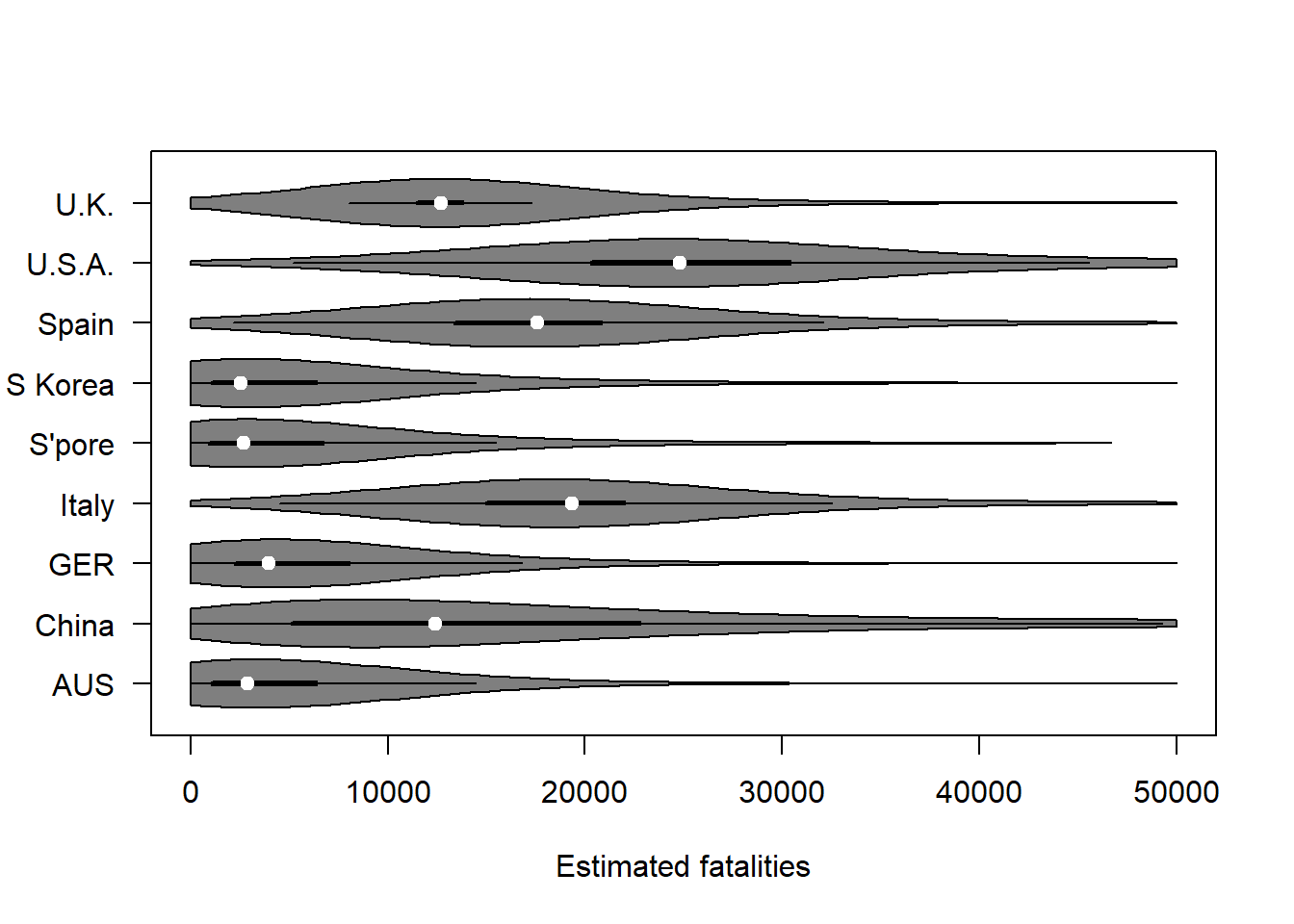
There are 4 items probing people’s COVID risk perception:
- How severe do you think novel coronavirus (COVID-19) will be in the population as a whole?
- How harmful would it be for your health if you were to become infected with COVID-19?
- How concerned are you that you might become infected with COVID-19?
- How concerned are you that somebody you know might become infected with novel?
Provide snapshot of responses and correlations between items.
covvars<-gather(covfin %>% select(c(COVID_gen_harm,COVID_pers_harm,COVID_pers_concern,COVID_concern_oth)),factor_key = TRUE)
covvars$key <- factor(covvars$key,labels=c("General harm","Personal harm","Concern self","Concern others"))
covhisto <- ggplot(covvars, aes(value)) +
  theme_classic() +
  theme(panel.grid.minor.y = element_line(colour="lightgray", size=0.5),
        panel.grid.major.y = element_line(colour="darkgray", size=0.5),
        panel.grid.major.x = element_blank(),
        panel.border = element_rect(colour = "black", size=1, fill=NA)) +
  geom_histogram(bins = 5, color="darkblue", fill="lightblue") +
  xlab("Response") + ylab("Frequency") +
  facet_wrap(~key, scales = 'free_x',labeller=label_value)
ggsave("covhisto.pdf")
Saving 7 x 5 in imageWarning: Removed 2 rows containing non-finite values (stat_bin).print(covhisto)Warning: Removed 2 rows containing non-finite values (stat_bin).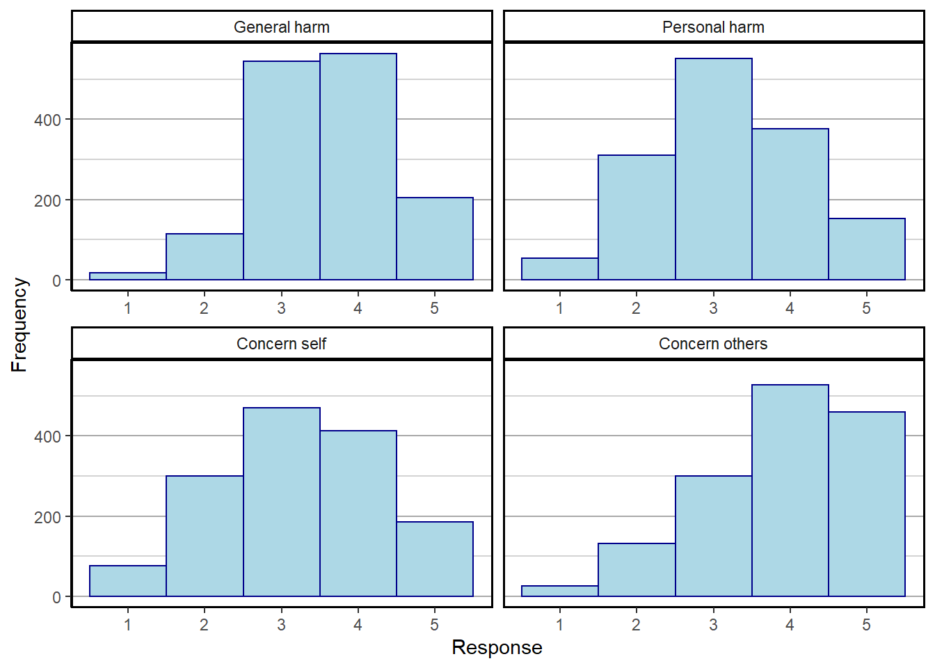
covfin %>% select(c(COVID_gen_harm,COVID_pers_harm,COVID_pers_concern,COVID_concern_oth)) %>% cor (.,use="pairwise.complete.obs") %>% round(.,3) COVID_gen_harm COVID_pers_harm COVID_pers_concern
COVID_gen_harm 1.000 0.351 0.414
COVID_pers_harm 0.351 1.000 0.626
COVID_pers_concern 0.414 0.626 1.000
COVID_concern_oth 0.421 0.409 0.668
COVID_concern_oth
COVID_gen_harm 0.421
COVID_pers_harm 0.409
COVID_pers_concern 0.668
COVID_concern_oth 1.000#compute composite score for COVID risk
covfin$COVIDrisk <- covfin %>% select(c(COVID_gen_harm,COVID_pers_harm,COVID_pers_concern,COVID_concern_oth)) %>% apply(.,1, mean, na.rm=TRUE)
#compute composite score for government trust
covfin$govtrust <- covfin %>% select(starts_with("trus")) %>% apply(.,1, mean, na.rm=TRUE)
###############################################################################################################3 Comparison between scenarios
3.1 Efficacy of policy
Not all items are entirely commensurate between scenarios. We begin with a graphical summary.
The figure below shows people’s confidence that each of the scenarios would reduce their likelihood of contracting COVID-19:
plotvio (covfin, c("reduce_lik_bt", "reduce_lik_mild","reduce_lik_sev" ), "blue", "Reduce contracting")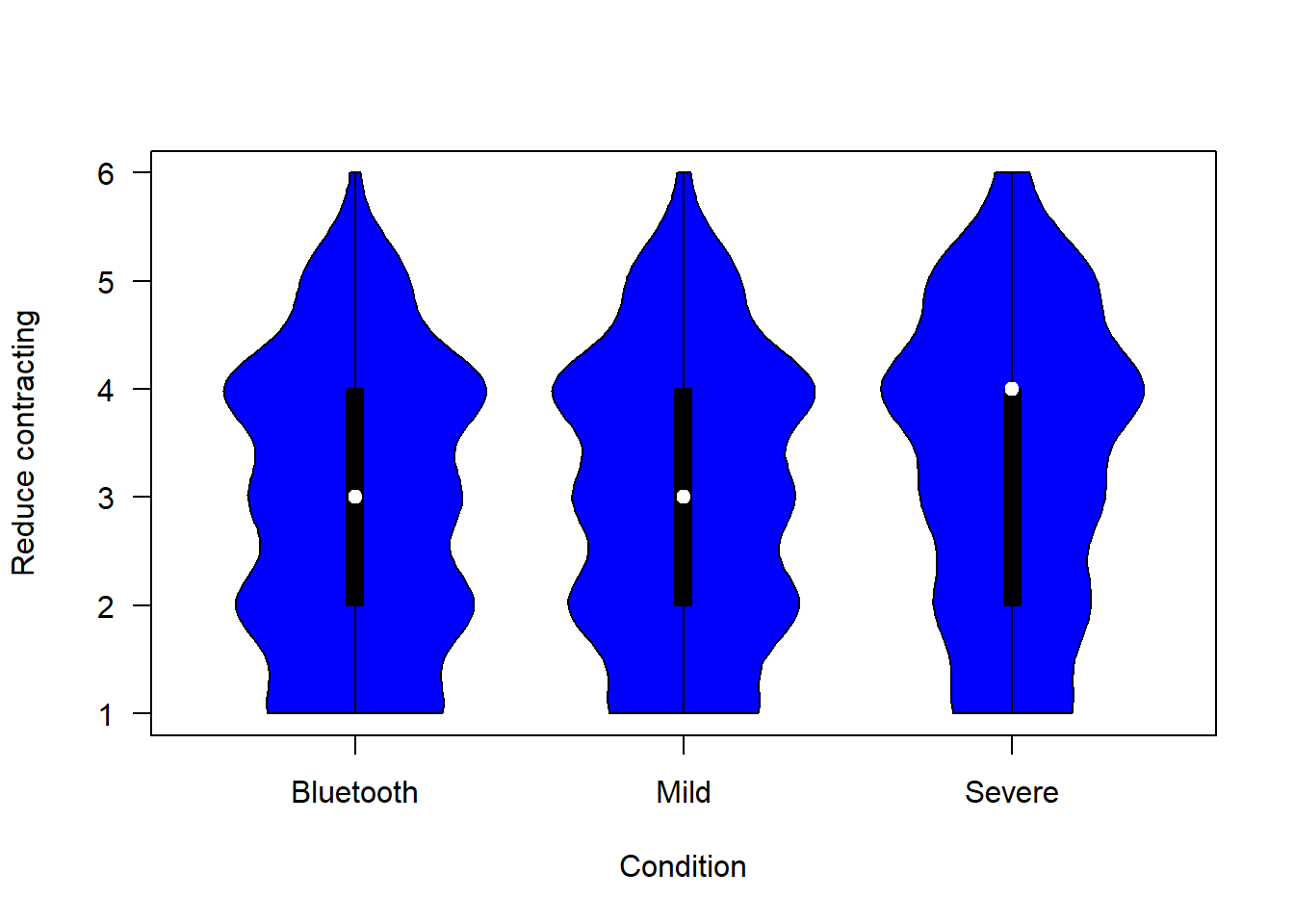
The figure below shows people’s confidence that each of the scenarios would allow them to resume their normal lives more rapidly
plotvio (covfin, c("return_activ_bt", "return_activ_mild", "return_activ_sev"), "green", "Resume normal")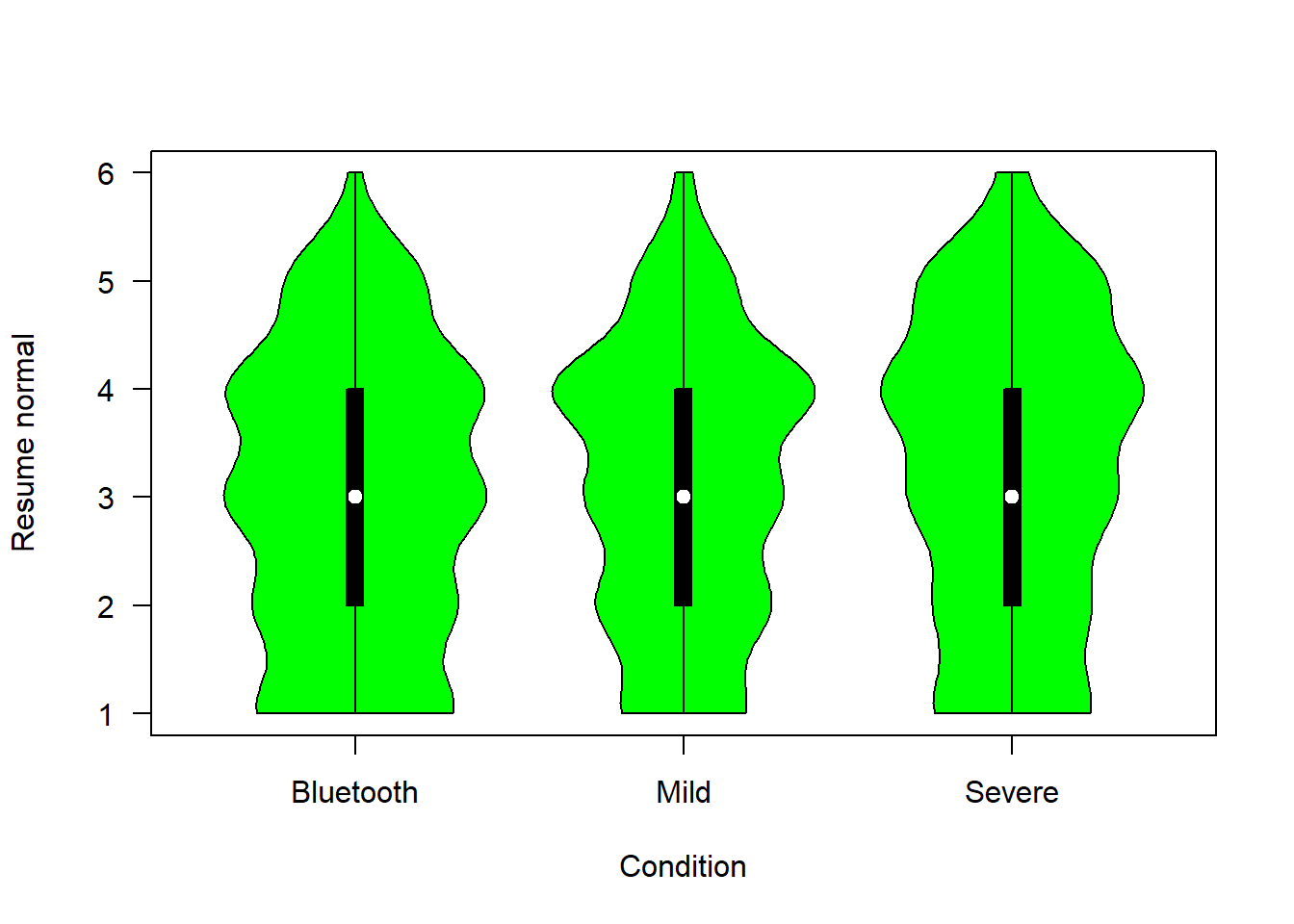
The figure below shows people’s confidence that each of the scenarios would reduce spread of COVID-19 in the community.
plotvio (covfin, c("reduce_spread_bt", "reduce_spread_mild", "reduce_spread_sev"), "orange", "Reduce spread")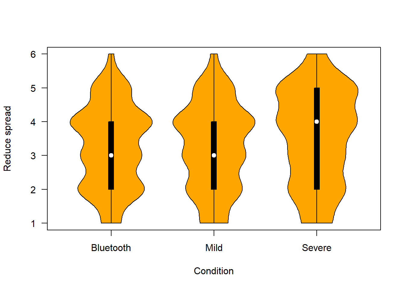
3.2 Acceptability of policy
Basic acceptability of each scenario, probed by a single item immediately after reading the scenario. The table shows percentages. For the mild and Bluetooth scenarios, the question refers to whether participant would download the app. For the severe scenario, the question refers to acceptability of the tracking mandated by government.
#use gather and drop
accept1 <- covfin %>% select(c(app_uptake1_mild, is_acceptable1_sev, bluetooth_uptake1_bt)) %>%
                    pivot_longer(c(app_uptake1_mild,is_acceptable1_sev,bluetooth_uptake1_bt),
                                names_to = "key", values_to = "value")
covfin$accept1 <- (accept1 %>% drop_na())$value
#we do not drop NAs for the pivoted data frame to allow correct merging with the conditional responses below for quasi interval score
accept1 <- apply_labels(accept1,
                        value = "Acceptability of policy",
                        value = c("Yes" = 1, "No" = 0),
                        key = "Type of scenario",
                        key = c("Mild" ="app_uptake1_mild", "Severe" = "is_acceptable1_sev", "Bluetooth" = "bluetooth_uptake1_bt"))
cro_tpct(accept1$value,row_vars=accept1$key) #presence of NAs makes no difference here| #Total | |||
|---|---|---|---|
| Type of scenario | |||
| Bluetooth | Acceptability of policy | No | 30.2 |
| Yes | 69.8 | ||
| #Total cases | 483 | ||
| Mild | Acceptability of policy | No | 30.8 |
| Yes | 69.2 | ||
| #Total cases | 477 | ||
| Severe | Acceptability of policy | No | 38.1 |
| Yes | 61.9 | ||
| #Total cases | 486 | ||
chisq.test(unlabel(accept1$value),unlabel(accept1$key),correct=TRUE)
    Pearson's Chi-squared test

data:  unlabel(accept1$value) and unlabel(accept1$key)
X-squared = 8.338, df = 2, p-value = 0.01547
The difference between acceptability of scenarios is significant by a \(\chi^2\) test on the contingency table.
Repeated probing of basic acceptability of each scenario after multiple questions about the scenario have been answered. The table shows percentages. For the mild and Bluetooth scenarios, the question refers to whether participant would download the app. For the severe scenario, the question refers to acceptability of the tracking mandated by government.
covfin$accept2 <- apply(cbind(covfin$app_uptake2_mild,covfin$is_acceptable2_sev,covfin$bluetooth_uptake2_bt),1,sum,na.rm=TRUE)
covfin <- apply_labels(covfin,
                        accept2 = "Acceptability of policy",
                        accept2 = c("Yes" = 1, "No" = 0),
                        scenario_type = "Type of scenario")
cro_tpct(covfin$accept2,row_vars=covfin$scenario_type)| #Total | |||
|---|---|---|---|
| Type of scenario | |||
| bluetooth | Acceptability of policy | No | 34.2 |
| Yes | 65.8 | ||
| #Total cases | 483 | ||
| mild | Acceptability of policy | No | 34.0 |
| Yes | 66.0 | ||
| #Total cases | 477 | ||
| severe | Acceptability of policy | No | 41.4 |
| Yes | 58.6 | ||
| #Total cases | 486 | ||
chisq.test(covfin$accept2,covfin$scenario_type,correct=TRUE)
    Pearson's Chi-squared test

data:  covfin$accept2 and covfin$scenario_type
X-squared = 7.4123, df = 2, p-value = 0.02457
The difference between acceptability of scenarios is again significant by a \(\chi^2\) test, and overall acceptability of all scenarios has been reduced slightly compared to first set of questions.
Those people who found the scenario unacceptable at the second opportunity were asked two follow-up questions. Those questions were as follows:
First, for both scenarios, people were asked if their decision would change if the government was required to delete the data and cease tracking after 6 months. Overall acceptance of the policies when a sunset clause was included was as follows:
covfin$accept3 <- apply(cbind(covfin$accept2,covfin %>% select(contains("sunset"))),1,sum,na.rm=TRUE)
covfin <- apply_labels(covfin,
                       accept3 = "Acceptability of policy",
                       accept3 = c("Yes" = 1, "No" = 0),
                       scenario_type = "Type of scenario")
cro_tpct(covfin$accept3,row_vars=covfin$scenario_type)| #Total | |||
|---|---|---|---|
| Type of scenario | |||
| bluetooth | Acceptability of policy | No | 28.6 |
| Yes | 71.4 | ||
| #Total cases | 483 | ||
| mild | Acceptability of policy | No | 24.1 |
| Yes | 75.9 | ||
| #Total cases | 477 | ||
| severe | Acceptability of policy | No | 24.9 |
| Yes | 75.1 | ||
| #Total cases | 486 | ||
chisq.test(covfin$accept3,covfin$scenario_type,correct=TRUE)
    Pearson's Chi-squared test

data:  covfin$accept3 and covfin$scenario_type
X-squared = 2.8496, df = 2, p-value = 0.2406###############################################################################################################The sunset clause uniformly increased acceptance of the scenarios, with no significant differences between them.
The second follow-up question differed between scenarios. People in the mild scenario were asked if they would change their decision if data was stored only on the user’s smartphone (not government servers), and people were given the option to provide the data if they tested positive. People in the severe scenario were asked if they would change their decision if there was an option to opt out of data collection. People in the Bluetooth scenario were not asked a second follow-up question (which is why there responses are unchanged below compared to the sunset responses).
covfin$accept5 <- apply(cbind(covfin$accept2,covfin %>% select(contains("sunset")),
                                      covfin$change_dlocal_mild,covfin$change_optout_sev),1,max,na.rm=TRUE)
covfin <- apply_labels(covfin,
                       accept5 = "Acceptability of policy",
                       accept5 = c("Yes" = 1, "No" = 0),
                       scenario_type = "Type of scenario")
cro_tpct(covfin$accept5,row_vars=covfin$scenario_type)| #Total | |||
|---|---|---|---|
| Type of scenario | |||
| bluetooth | Acceptability of policy | No | 28.6 |
| Yes | 71.4 | ||
| #Total cases | 483 | ||
| mild | Acceptability of policy | No | 16.6 |
| Yes | 83.4 | ||
| #Total cases | 477 | ||
| severe | Acceptability of policy | No | 11.3 |
| Yes | 88.7 | ||
| #Total cases | 486 | ||
chisq.test(covfin$accept5,covfin$scenario_type,correct=TRUE)
    Pearson's Chi-squared test

data:  covfin$accept5 and covfin$scenario_type
X-squared = 49.581, df = 2, p-value = 1.712e-11###############################################################################################################The opt-out/local storage options further enhanced acceptance.
3.3 Assessment of risk of scenarios, trust in government / Apple and Google and data security
How difficult is it for people to decline participation in the proposed project? (1 = Extremely easy – 6 = Extremely difficult)
  covfin$decline_participate[covfin$scenario_type=="bluetooth"] <- covfin$decline_part_bt[covfin$scenario_type=="bluetooth"]
  vioplot(decline_participate ~ scenario_type, data=covfin, col = "lightgray", ylab="Decline", xlab="Condition", las=1, )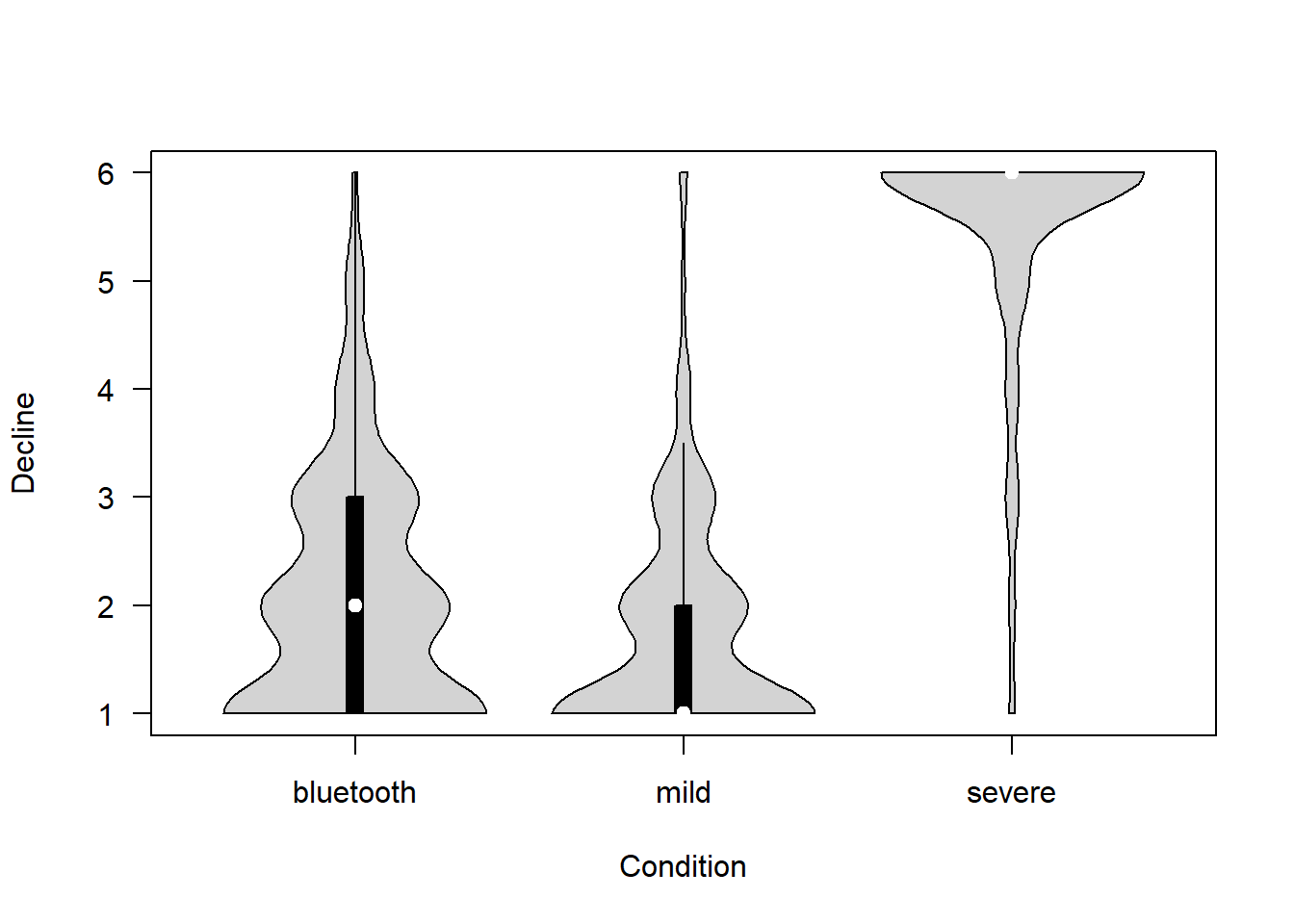
To what extent is the Government only collecting the data necessary? (1 = Not at all – 6 = Completely)
  covfin$proportionality[covfin$scenario_type=="bluetooth"] <- covfin$proportionality_bt[covfin$scenario_type=="bluetooth"]
  vioplot(proportionality ~ scenario_type, data=covfin, col = "lightgray", ylab="Only data necessary", xlab="Condition", las=1, )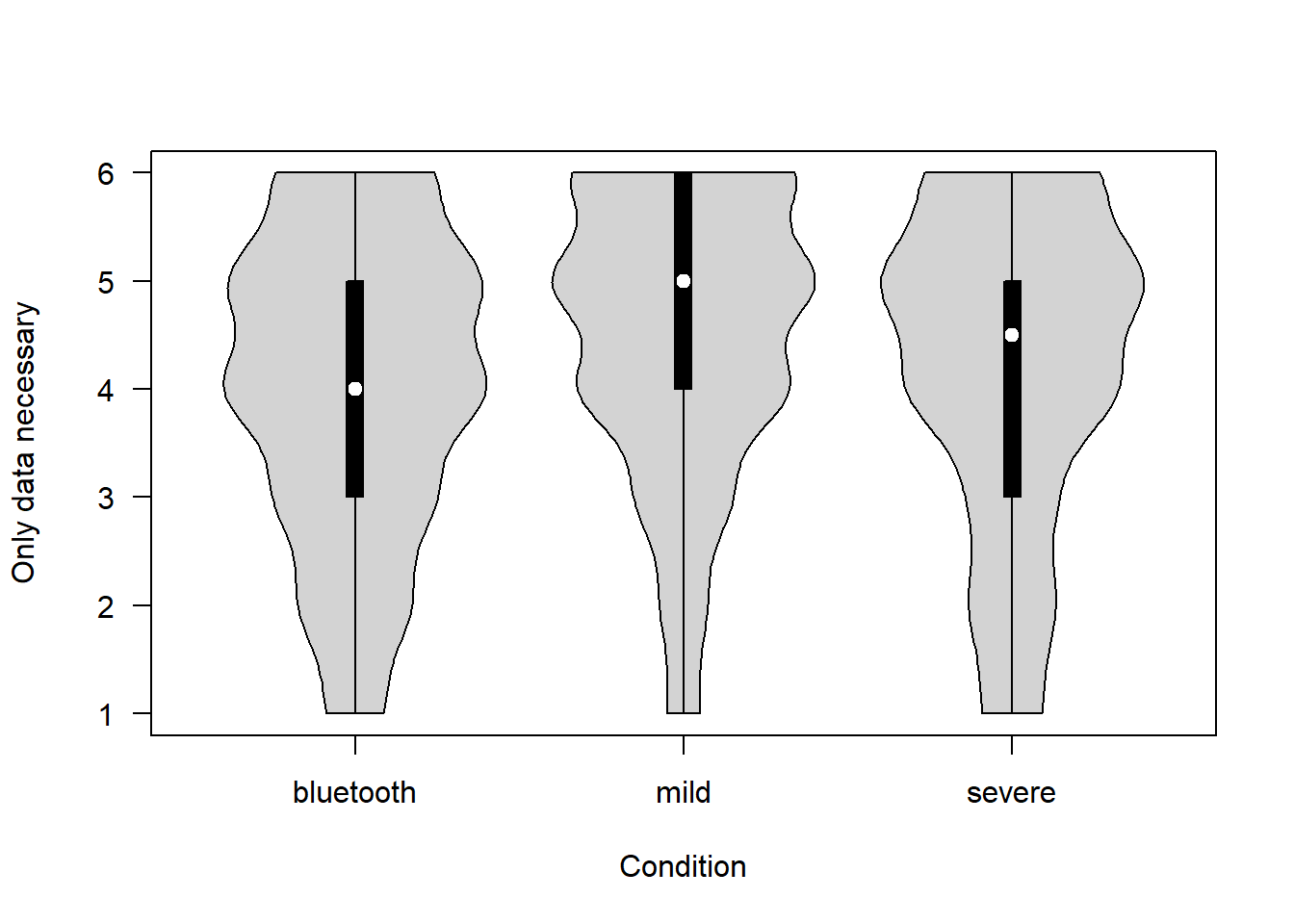
How sensitive is the data being collected in the proposed project? (1 = Not at all – 6 = Extremely)
  covfin$sensitivity[covfin$scenario_type=="bluetooth"] <- covfin$sensitivity_bt[covfin$scenario_type=="bluetooth"]
  vioplot(sensitivity ~ scenario_type, data=covfin, col = "lightgray", ylab="Sensitivity of data", xlab="Condition", las=1, )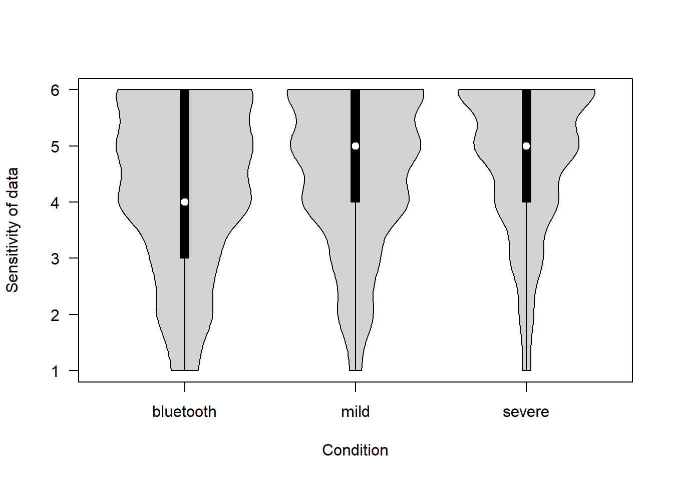
How serious is the risk of harm that could arise from the proposed project? (1 = Not at all – 6 = Extremely)
  covfin$risk_of_harm[covfin$scenario_type=="bluetooth"] <- covfin$risk_of_harm_bt[covfin$scenario_type=="bluetooth"]
  vioplot(risk_of_harm ~ scenario_type, data=covfin, col = "lightgray", ylab="Risk of harm", xlab="Condition", las=1, )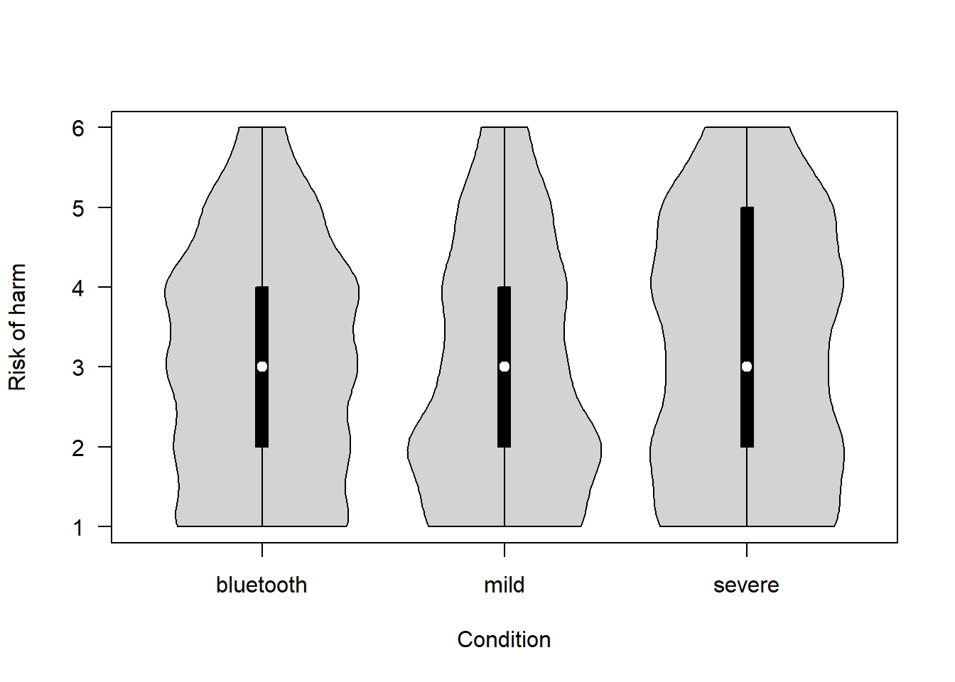
How much do you trust the Government (or Apple and Google in the Bluetooth scenario) to use the tracking data only to deal with the COVID-19 pandemic? (1 = Not at all – 6 = Completely)
  covfin$trust_intentions[covfin$scenario_type=="bluetooth"] <- covfin$trust_intentions_bt[covfin$scenario_type=="bluetooth"]
  vioplot(trust_intentions ~ scenario_type, data=covfin, col = "lightgray", ylab="Trust intentions of government/corporations", xlab="Condition", las=1, )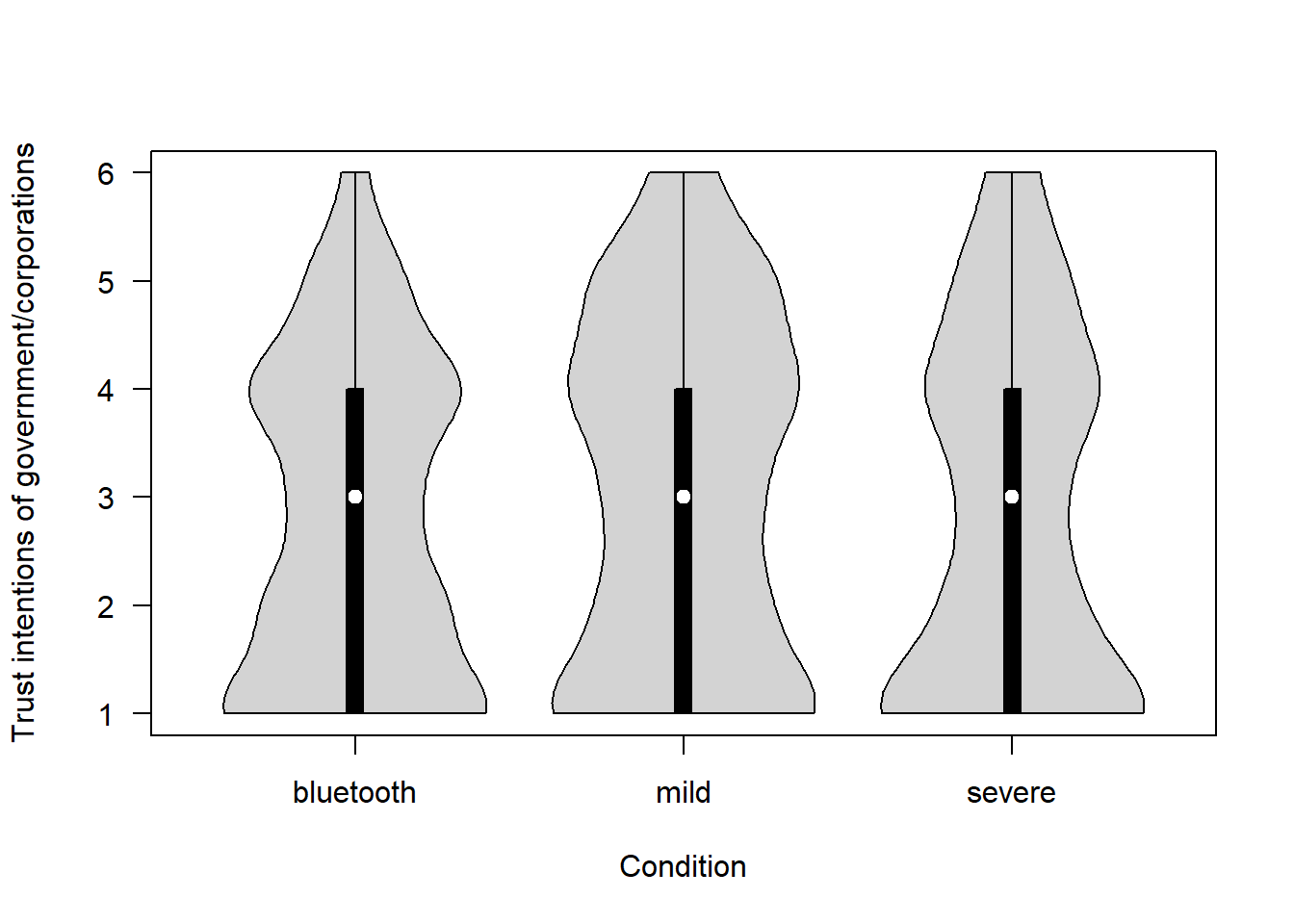
How much do you trust the Government (or Apple and Google in the Bluetooth scenario) to be able to ensure the privacy of each individual? (1 = Not at all – 6 = Completely)
  covfin$trust_respect_priv[covfin$scenario_type=="bluetooth"] <- covfin$trust_respectpriv_bt[covfin$scenario_type=="bluetooth"]
  vioplot(trust_respect_priv ~ scenario_type, data=covfin, col = "lightgray", ylab="Trust government/corporations preserve privacy", xlab="Condition", las=1, )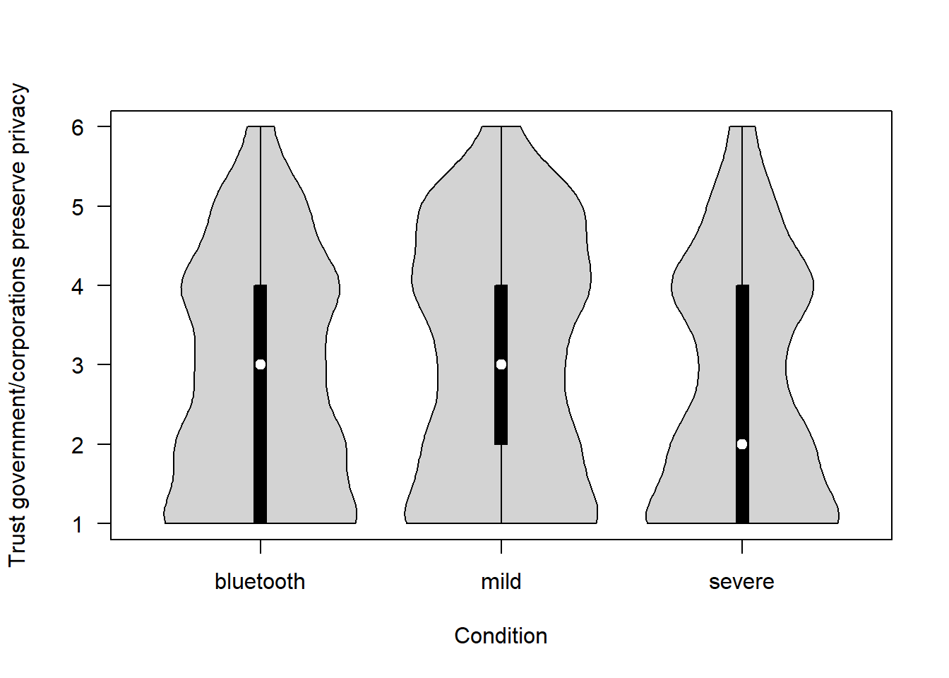
How secure is the data that would be collected for the proposed project? (1 = Not at all – 6 = Completely)
  covfin$data_security[covfin$scenario_type=="bluetooth"] <- covfin$data_security_bt[covfin$scenario_type=="bluetooth"]
  vioplot(data_security ~ scenario_type, data=covfin, col = "lightgray", ylab="How secure is data", xlab="Condition", las=1, )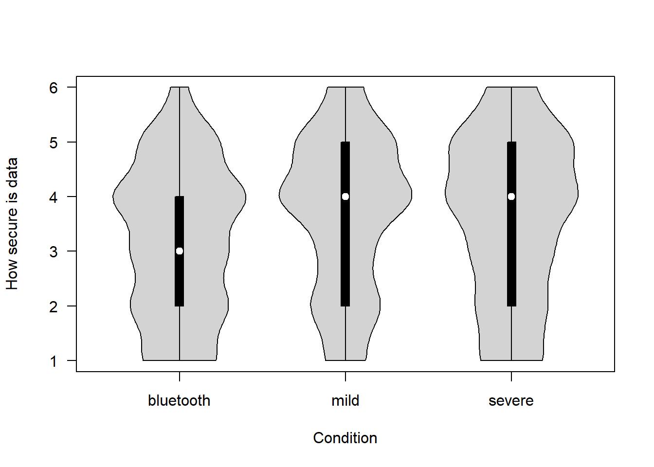
To what extent do people have ongoing control of their data? (1 = No control at all – 6 = Complete control)
vioplot(ongoing_control ~ scenario_type, data=covfin, col = "lightgray", ylab="Ongoing control over data", xlab="Condition", las=1, )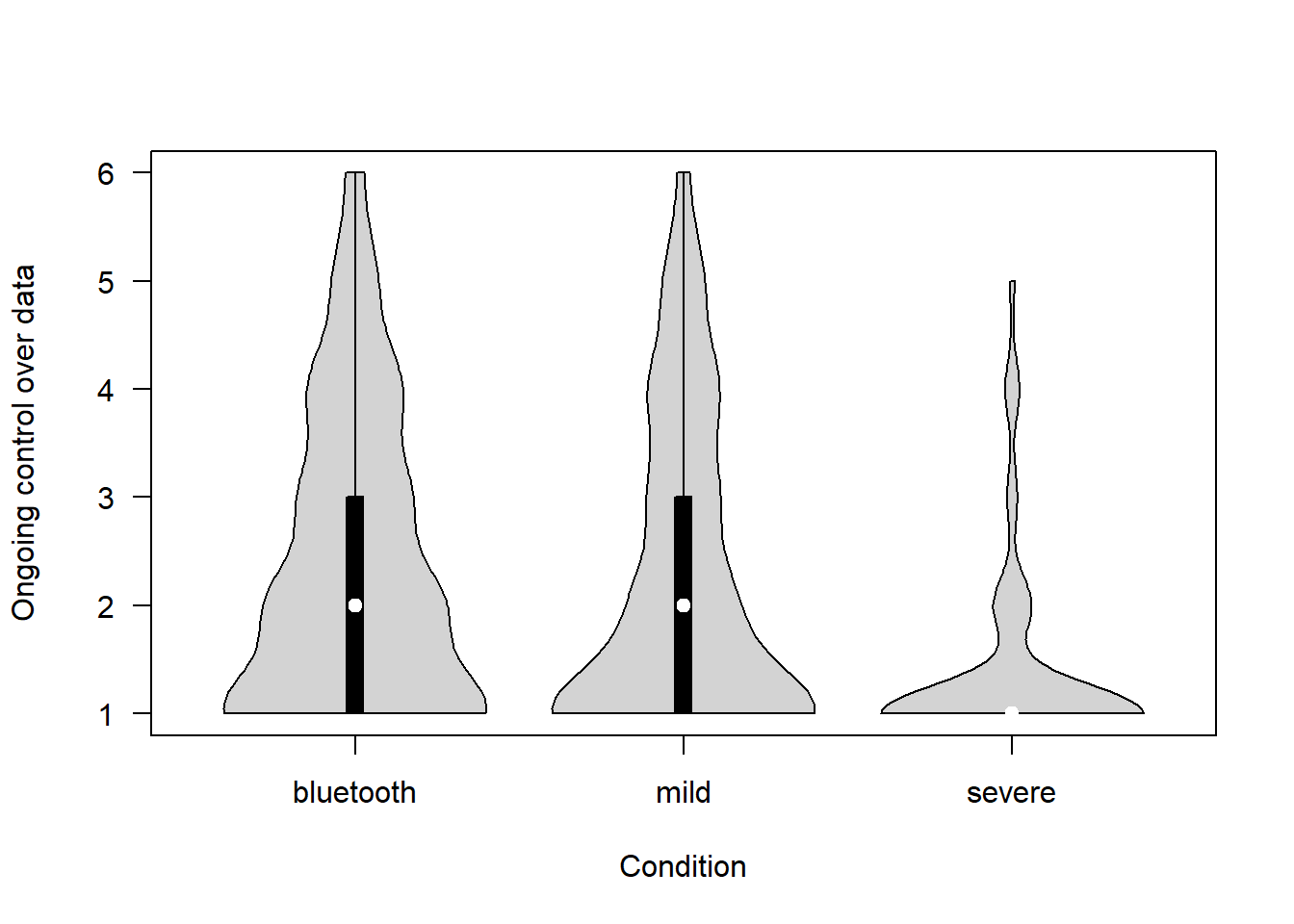
4 Role of worldviews
4.1 Worldview and risk perception
We relate a composite of the 3 worldview items to the composite of the 4 items probing perceived risk from COVID. Worldview is scored such that greater values reflect greater libertarianism.
p <- ggplot(covfin, aes(Worldview, COVIDrisk)) +
  geom_point(size=1.5,shape = 21,fill="red",
             position=position_jitter(width=0.15, height=0.15)) +
  geom_smooth() +
  theme(plot.title = element_text(size = 18),
        panel.background = element_rect(fill = "white", colour = "grey50"),
        text = element_text(size=14)) +
  xlim(0.8,7.2) + ylim(0.8,5.2) +
  labs(x="Worldview (libertarianism)", y="Perceived COVID risk")
print(p)
`geom_smooth()` using method = 'gam' and formula 'y ~ s(x, bs = "cs")'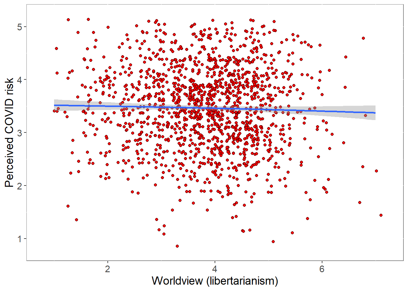
pcor <- cor.test (covfin$Worldview,covfin$COVIDrisk, use="pairwise.complete.obs") %>% print()
    Pearson's product-moment correlation

data:  covfin$Worldview and covfin$COVIDrisk
t = -1.6796, df = 1444, p-value = 0.09326
alternative hypothesis: true correlation is not equal to 0
95 percent confidence interval:
 -0.095488518  0.007411261
sample estimates:
        cor
-0.04415574 ###############################################################################################################There is no evidence for an association between libertarianism and risk perception.
4.2 Worldviews and trust
We relate the composite of the 3 worldview items to the composite of the two trust-in-government items (which correlate 0.838 for severe and mild, and 0.815 for the Bluetooth scenario).
p <- ggplot(covfin, aes(Worldview, govtrust)) +
  geom_point(size=1.5,shape = 21,fill="red",
             position=position_jitter(width=0.15, height=0.15)) +
  geom_smooth() +
  theme(plot.title = element_text(size = 18),
        panel.background = element_rect(fill = "white", colour = "grey50"),
        text = element_text(size=14)) +
  xlim(0.8,7.2) + ylim(0.8,5.2) +
  labs(x="Worldview (libertarianism)", y="Trust in government")
print(p)
`geom_smooth()` using method = 'gam' and formula 'y ~ s(x, bs = "cs")'Warning: Removed 66 rows containing non-finite values (stat_smooth).Warning: Removed 66 rows containing missing values (geom_point).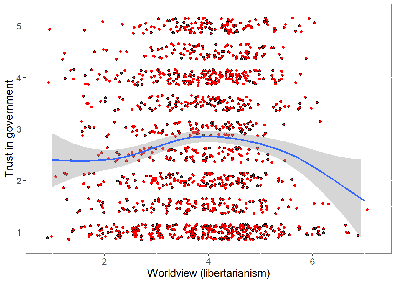
pcor <- cor.test (covfin$Worldview,covfin$govtrust, use="pairwise.complete.obs") %>% print()
    Pearson's product-moment correlation

data:  covfin$Worldview and covfin$govtrust
t = 1.6982, df = 1444, p-value = 0.08969
alternative hypothesis: true correlation is not equal to 0
95 percent confidence interval:
 -0.006921978  0.095973343
sample estimates:
       cor
0.04464408 ###############################################################################################################The pattern is not straightforward and may not be linear, but there is some evidence that trust is reduced among extreme libertarians.
5 Immunity Passports
Participants were asked their views on “immunity passports”, explained as follows:
An ‘immunity passport’ indicates that you have had a disease and that you have the antibodies for the virus causing that disease. Having the antibodies implies that you are now immune and therefore unable to spread the virus to other people. Thus, if an antibody test indicates that you have had the disease, you could be allocated an ‘immunity passport’ which would subsequently allow you to move around freely. Immunity passports have been proposed as a potential step towards lifting movement restrictions during the COVID-19 pandemic.
5.1 Basic summary of immunity passport items
There were 7 items that queries attitudes towards immunity passports:
Would you support a government proposal to introduce ‘immunity passports’ for novel coronavirus (COVID-19)? (1 = Not at all – 6 = Fully)
How concerned are you about the idea of introducing an ‘immunity passport’ for novel coronavirus (COVID-19)? (1 = Not at all – 5 = Extremely)
How much would you like to be allocated an ‘immunity passport’ for novel coronavirus (COVID-19)? (1 = Not at all – 6 = Extremely)
To what extent do you believe an ‘immunity passport’ for novel coronavirus (COVID-19) could harm the social fabric of your country? (1 = Not at all – 6 = Extremely)
To what extent do you believe that it is fair for people with ‘immunity passports’ for novel coronavirus (COVID-19) to go back to work, while individuals without such an ‘immunity passport’ cannot? (Extremely unfair = 1 – Extemely fair = 6)
To what extent would you consider purposefully infecting yourself with novel coronavirus (COVID-19) to get an ‘immunity passport’ for novel coronavirus (COVID-19)? (1 = Not at all – 6 = Extremely)
Would you support a government proposal to introduce ‘immunity passports’ for novel coronavirus (COVID-19)? (1 = Not at all – 6 = Fully)
Summary statistics for the 7 items are:
ipcov <- covfin %>% select(starts_with("ip_"))

hist(ipcov)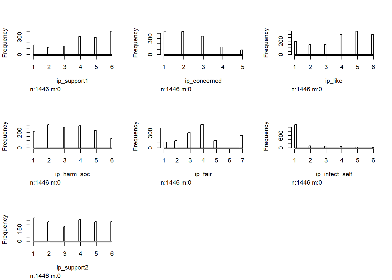
ipcov <- apply_labels(ipcov,ip_support2 = "Final support for Immunity Passports",
                            ip_support2 = c("Not at all" = 1, "Slightly" = 2, "A bit" = 3,
                                            "Moderately" = 4, "A lot" = 5, "Fully" = 6))
cro_tpct(ipcov$ip_support2)| #Total | |
|---|---|
| Final support for Immunity Passports | |
| Not at all | 19.8 |
| Slightly | 16.6 |
| A bit | 12.4 |
| Moderately | 18.2 |
| A lot | 16.5 |
| Fully | 16.5 |
| #Total cases | 1446 |
Around 20% of participants reject the idea of immunity passports whereas more than 30% strongly or fully endorse it.
Two of the items (concern and fairness), are now reverse scored so everything is pointing in the same direction. Correlations among items are shown first, followed by graphs relating a composite immunity-passport-endorsement score to other variables. (Note: this is a crude composite score because scales with a different number of points are combined. This needs to be fixed.)
ipcov %<>% mutate(ip_concerned = revscore(ip_concerned,5), ip_harm_soc  = revscore(ip_harm_soc,6)) %>% select(-ip_infect_self)

cor(ipcov)
ip_support1 ip_concerned ip_like ip_harm_soc ip_fair
ip_support1 1.0000000 0.6702438 0.7558093 0.6025573 0.5698996
ip_concerned 0.6702438 1.0000000 0.5499829 0.6432464 0.4707144
ip_like 0.7558093 0.5499829 1.0000000 0.4493977 0.4893675
ip_harm_soc 0.6025573 0.6432464 0.4493977 1.0000000 0.5069048
ip_fair 0.5698996 0.4707144 0.4893675 0.5069048 1.0000000
ip_support2 0.8453319 0.6258621 0.7369978 0.6223460 0.6272880
ip_support2
ip_support1 0.8453319
ip_concerned 0.6258621
ip_like 0.7369978
ip_harm_soc 0.6223460
ip_fair 0.6272880
ip_support2 1.0000000covfin$ipendorse <- apply(ipcov,1,mean,na.rm=TRUE)
p <- ggplot(covfin, aes(Worldview, ipendorse)) +
geom_point(size=1.5,shape = 21,fill="red",
position=position_jitter(width=0.15, height=0.15)) +
geom_smooth() +
theme(plot.title = element_text(size = 18),
panel.background = element_rect(fill = "white", colour = "grey50"),
text = element_text(size=14)) +
xlim(0.8,7.2) + ylim(0.8,5.2) +
labs(x="Worldview (libertarianism)", y="Endorsement of immunity passports")
print(p)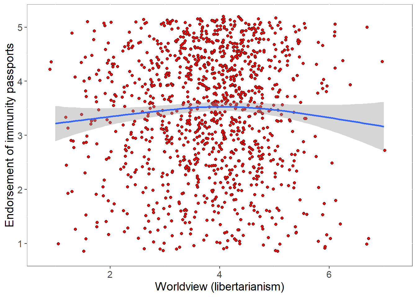
pcor <- cor.test (covfin$Worldview,covfin$ipendorse, use="pairwise.complete.obs") %>% print()
    Pearson's product-moment correlation

data:  covfin$Worldview and covfin$ipendorse
t = 1.7919, df = 1444, p-value = 0.07336
alternative hypothesis: true correlation is not equal to 0
95 percent confidence interval:
 -0.004457595  0.098414524
sample estimates:
       cor
0.04710336
p <- ggplot(covfin, aes(govtrust, ipendorse)) +
geom_point(size=1.5,shape = 21,fill="red",
position=position_jitter(width=0.15, height=0.15)) +
geom_smooth() +
theme(plot.title = element_text(size = 18),
panel.background = element_rect(fill = "white", colour = "grey50"),
text = element_text(size=14)) +
xlim(0.8,7.2) + ylim(0.8,5.2) +
labs(x="Trust in government", y="Endorsement of immunity passports")
print(p)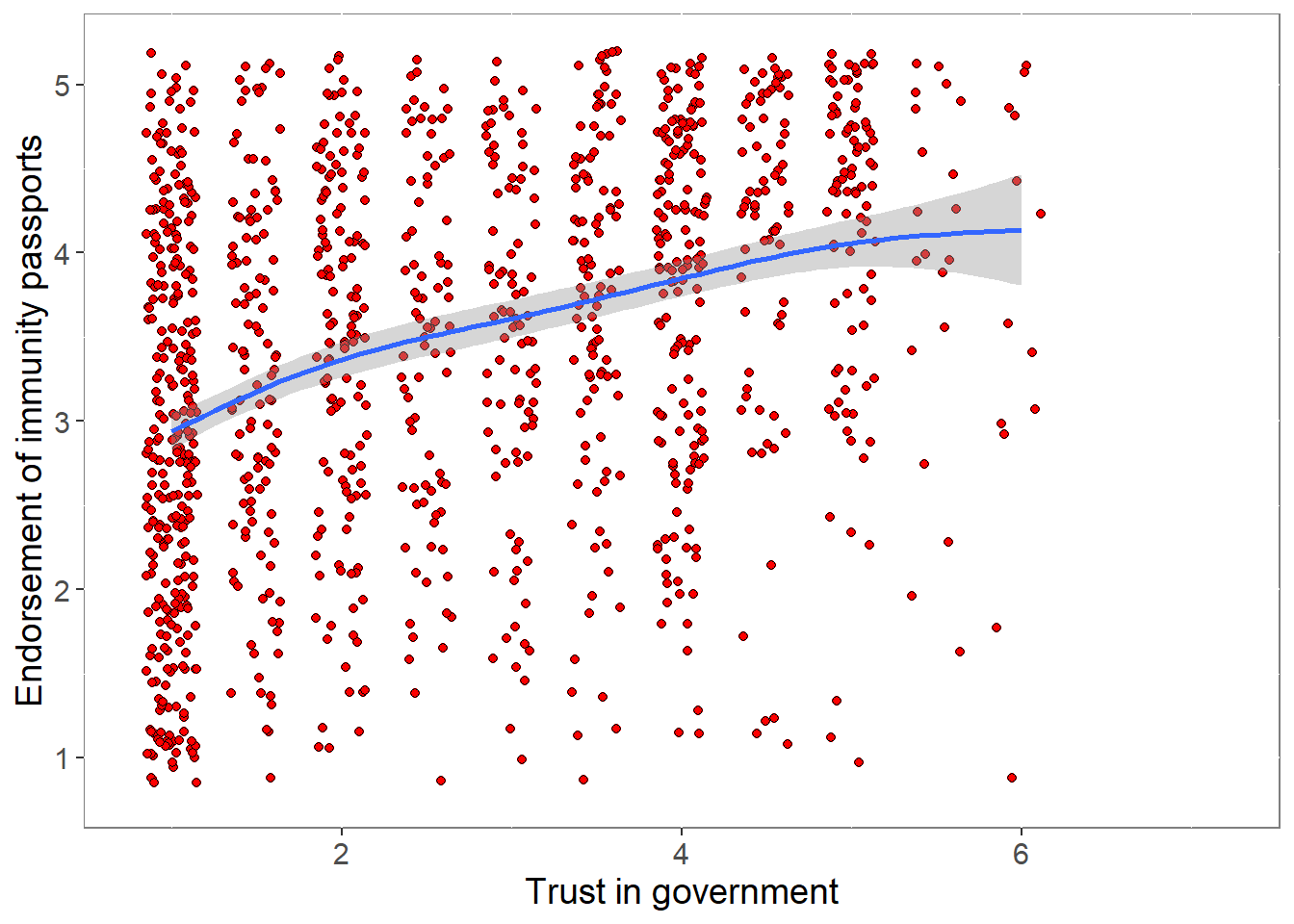
pcor <- cor.test (covfin$govtrust,covfin$ipendorse, use="pairwise.complete.obs") %>% print()
    Pearson's product-moment correlation

data:  covfin$govtrust and covfin$ipendorse
t = 15.662, df = 1444, p-value < 2.2e-16
alternative hypothesis: true correlation is not equal to 0
95 percent confidence interval:
 0.3361219 0.4242846
sample estimates:
      cor
0.3810692
p <- ggplot(covfin, aes(COVIDrisk,ipendorse)) +
geom_point(size=1.5,shape = 21,fill="red",
position=position_jitter(width=0.15, height=0.15)) +
geom_smooth() +
theme(plot.title = element_text(size = 18),
panel.background = element_rect(fill = "white", colour = "grey50"),
text = element_text(size=14)) +
xlim(0.8,7.2) + ylim(0.8,5.2) +
labs(y="Endorsement of immunity passports", x="Perceived COVID risk")
print(p)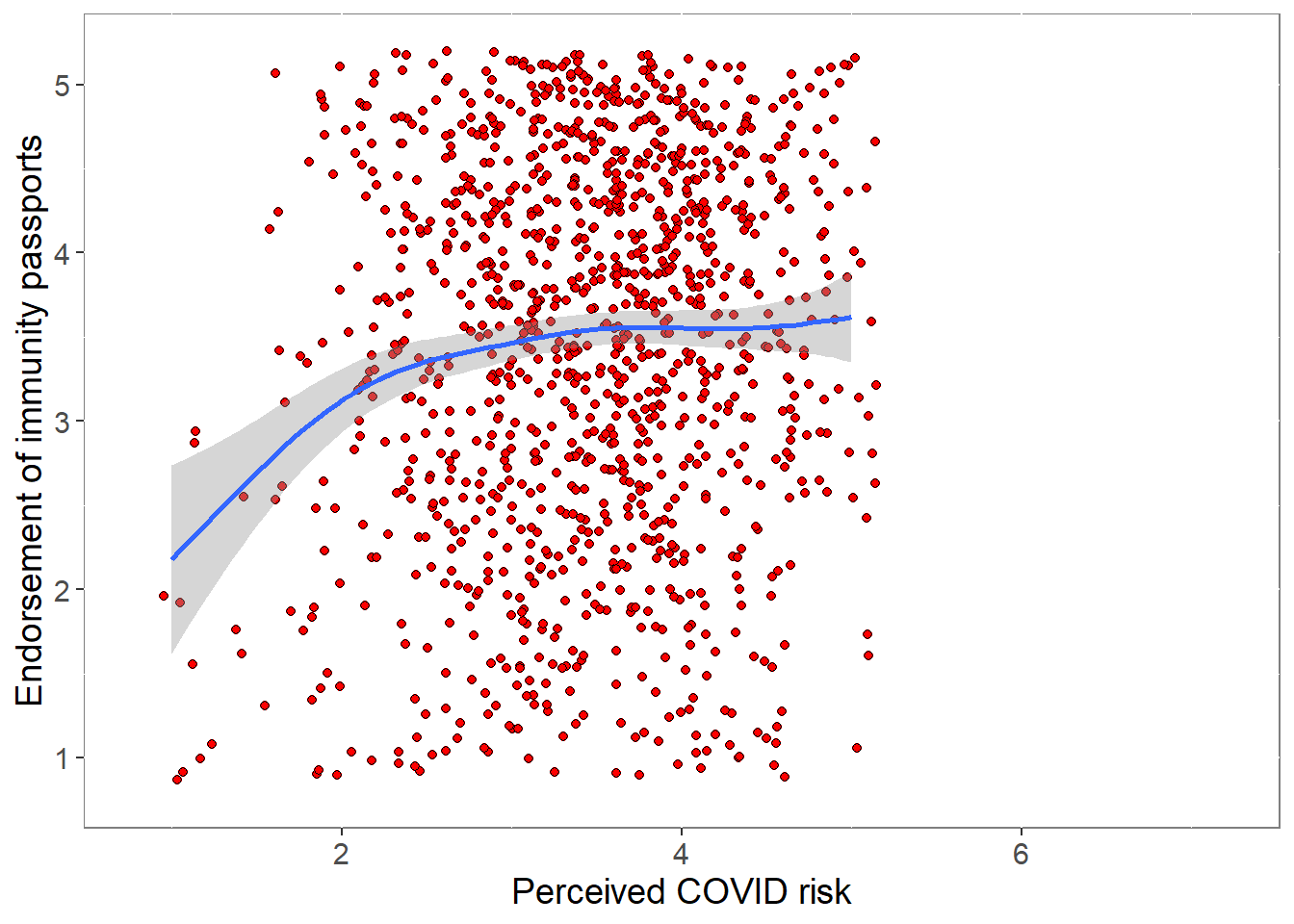
pcor <- cor.test (covfin$ipendorse,covfin$COVIDrisk, use="pairwise.complete.obs") %>% print()
    Pearson's product-moment correlation

data:  covfin$ipendorse and covfin$COVIDrisk
t = 4.0441, df = 1444, p-value = 5.529e-05
alternative hypothesis: true correlation is not equal to 0
95 percent confidence interval:
 0.05457475 0.15652339
sample estimates:
      cor
0.1058272
R version 3.6.3 (2020-02-29)
Platform: x86_64-w64-mingw32/x64 (64-bit)
Running under: Windows 10 x64 (build 19042)

Matrix products: default

locale:
[1] LC_COLLATE=English_United Kingdom.1252
[2] LC_CTYPE=English_United Kingdom.1252
[3] LC_MONETARY=English_United Kingdom.1252
[4] LC_NUMERIC=C
[5] LC_TIME=English_United Kingdom.1252

attached base packages:
[1] stats     graphics  grDevices utils     datasets  methods   base

other attached packages:
 [1] broom.mixed_0.2.4  kableExtra_1.2.1   jtools_2.0.3       expss_0.10.2
 [5] vioplot_0.3.4      zoo_1.8-7          sm_2.2-5.6         readxl_1.3.1
 [9] summarytools_0.9.6 scales_1.1.0       psych_1.9.12.31    reshape2_1.4.4
[13] Hmisc_4.4-0        Formula_1.2-3      survival_3.2-3     gridExtra_2.3
[17] lme4_1.1-21        Matrix_1.2-18      forcats_0.5.0      stringr_1.4.0
[21] dplyr_0.8.5        purrr_0.3.4        readr_1.3.1        tidyr_1.0.2
[25] tibble_3.0.1       ggplot2_3.3.0      tidyverse_1.3.0    stargazer_5.2.2
[29] hexbin_1.28.1      lattice_0.20-41    knitr_1.30         workflowr_1.6.1

loaded via a namespace (and not attached):
 [1] minqa_1.2.4         colorspace_1.4-1    pryr_0.1.4
 [4] ellipsis_0.3.0      rprojroot_1.3-2     htmlTable_1.13.3
 [7] base64enc_0.1-3     fs_1.4.1            rstudioapi_0.11
[10] farver_2.0.3        fansi_0.4.1         lubridate_1.7.8
[13] xml2_1.3.2          codetools_0.2-16    splines_3.6.3
[16] mnormt_1.5-6        jsonlite_1.6.1      nloptr_1.2.2.1
[19] broom_0.5.5         cluster_2.1.0       dbplyr_1.4.2
[22] png_0.1-7           compiler_3.6.3      httr_1.4.1
[25] backports_1.1.6     assertthat_0.2.1    cli_2.0.2
[28] later_1.0.0         acepack_1.4.1       htmltools_0.4.0
[31] tools_3.6.3         coda_0.19-3         gtable_0.3.0
[34] glue_1.4.1          Rcpp_1.0.4.6        cellranger_1.1.0
[37] vctrs_0.2.4         nlme_3.1-145        xfun_0.20
[40] rvest_0.3.5         lifecycle_0.2.0     MASS_7.3-51.5
[43] hms_0.5.3           promises_1.1.0      parallel_3.6.3
[46] TMB_1.7.16          RColorBrewer_1.1-2  yaml_2.2.1
[49] pander_0.6.3        rpart_4.1-15        latticeExtra_0.6-29
[52] stringi_1.4.6       checkmate_2.0.0     boot_1.3-24
[55] rlang_0.4.6         pkgconfig_2.0.3     matrixStats_0.56.0
[58] evaluate_0.14       labeling_0.3        rapportools_1.0
[61] htmlwidgets_1.5.1   tidyselect_1.0.0    plyr_1.8.6
[64] magrittr_1.5        R6_2.4.1            magick_2.3
[67] generics_0.0.2      DBI_1.1.0           mgcv_1.8-31
[70] pillar_1.4.3        haven_2.2.0         whisker_0.4
[73] foreign_0.8-76      withr_2.2.0         nnet_7.3-13
[76] modelr_0.1.6        crayon_1.3.4        rmarkdown_2.6
[79] jpeg_0.1-8.1        grid_3.6.3          data.table_1.12.8
[82] git2r_0.26.1        webshot_0.5.2       reprex_0.3.0
[85] digest_0.6.25       httpuv_1.5.2        munsell_0.5.0
[88] viridisLite_0.3.0   tcltk_3.6.3